2.3 — Multilayer Perceptrons, Features, and Superposition
Module 2 — The Transformer
From a contextual vector to a new contribution
Attention gives a token position access to information from permitted positions. The position-wise multilayer perceptron, or MLP, provides another kind of computation: it transforms a vector through a wider collection of nonlinear responses and writes a vector back into the residual stream.
You already calculated an affine–nonlinear–affine network in Lesson 1.3. We will not repeat its introduction to multiplication or training. Instead, we will ask what changes when that network becomes a component inside a Transformer, and why observing its hidden units is harder to interpret than computing them.
A tempting picture gives each unit a label: one for geography, another for quotation marks, another for Python. Sometimes a unit responds selectively enough to support a useful description. But the architecture supplies numerical coordinates, not a guaranteed inventory of concepts. A feature can involve several coordinates, and one coordinate can participate in several features. We need language that separates those possibilities before interpreting an activation plot.
By the end, you should be able to:
- trace an MLP from residual-width input through hidden expansion to residual-width output;
- distinguish a unit’s incoming response from its outgoing contribution;
- separate units, feature directions, distributed representations, polysemanticity, and superposition;
- calculate when a small overcomplete representation succeeds and when information is lost;
- make a bounded claim from contrasting activations and describe stronger evidence it would require.
The prerequisites are Lesson 1.3, the residual stream, and attention.
Needed now: matrix shapes, dot products, affine maps, coordinatewise nonlinear functions, and vector addition. We use individual column vectors, as in Lesson 1.3.
Useful refresh: a basis gives independent coordinate directions; a linear combination adds scaled vectors; orthogonal vectors have zero dot product. A collection of directions need not be a basis.
Side trail: matrix rank, compressed sensing, and dictionary-learning objectives. The examples need only elementary arithmetic; training sparse autoencoders belongs to Lesson 5.2.
A shared transformation at every position
Let \(x_i\in\mathbb{R}^{d}\) be the residual vector immediately before a sequential pre-norm MLP branch at position \(i\). Its actual input is \(u_i=N(x_i)\), where \(N\) is that branch’s normalization. Define
\[ \begin{aligned} z_i&=W_{\mathrm{in}}u_i+b_{\mathrm{in}},\\ h_i&=\phi(z_i),\\ \Delta_i&=W_{\mathrm{out}}h_i+b_{\mathrm{out}},\\ y_i&=x_i+\Delta_i. \end{aligned} \]
Here \(z_i\) is the preactivation, \(h_i\) the post-activation hidden vector, and \(\Delta_i\) the MLP’s residual contribution. The last line is the surrounding residual addition, not another operation hidden inside the MLP. We inspect evaluation-time computation with dropout disabled.
For hidden width \(m\),
\[ W_{\mathrm{in}}\in\mathbb{R}^{m\times d},\quad b_{\mathrm{in}}\in\mathbb{R}^{m},\quad W_{\mathrm{out}}\in\mathbb{R}^{d\times m},\quad b_{\mathrm{out}}\in\mathbb{R}^{d}. \]
Thus the branch changes width \(d\rightarrow m\rightarrow d\). Biases may be absent in particular architectures. The output returns to \(d\) because it must be added to \(x_i\). Hidden width is neither sequence length nor vocabulary size.
The same matrices and biases apply at every position within this MLP. Different blocks generally have different parameters. No displayed equation reads \(u_j\) for a different position \(j\): the MLP does not itself transport information across positions. Nevertheless, \(u_i\) can already contain information gathered from the prefix. Position-wise computation can therefore respond to context without directly looking up another row.
The original Transformer’s feedforward component uses this two-affine-map pattern with ReLU, residual width 512, and hidden width 2048. Its normalization is after residual addition, unlike our pre-norm illustration. The shared position-wise operation and the surrounding topology are separate choices. Vaswani and colleagues, Sections 3.1 and 3.3
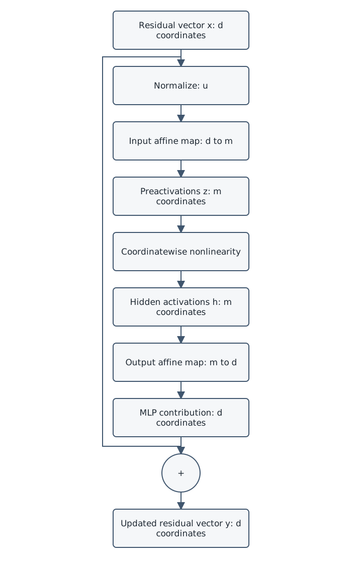
Original course diagram of one position’s sequential pre-norm MLP branch. Repeat the same branch at each position with shared parameters.
Prose alternative: Keep the original residual vector for the skip path. Normalize another copy, expand it to the hidden width, apply the nonlinearity to each hidden coordinate, and project back to residual width. Add that contribution to the original residual vector. The expanded vector is an intermediate activation, not a wider residual stream.
Expansion gives more nonlinear responses
A wider hidden layer provides more input-weight vectors and nonlinear response functions before the branch combines their outputs. It does not create new independent information from nowhere. Every hidden value remains a function of the supplied \(u_i\) and stored parameters.
Without a nonlinearity, the two affine maps collapse into one affine map, as you derived in Lesson 1.3. With ReLU, different inputs can select different sets of positive responses. Increasing \(m\) offers more such responses, though actual capabilities depend on the trained parameters and the rest of the network. Width alone neither counts learned concepts nor guarantees their independence.
For this two-matrix form, the weight count is \(2dm\), plus \(m+d\) biases when present. Doubling \(m\) doubles the matrix-weight count. That makes hidden expansion a substantial resource choice. It is not a free way to add features, and the common ratio \(m/d=4\) is a configuration choice rather than a law.
We will keep activation variants brief. ReLU clips negative inputs to zero. GELU, used in the optional Lab’s checkpoint, smoothly rescales its input; in its exact mathematical form, \(\operatorname{GELU}(t)=t\Phi(t)\), with \(\Phi\) the standard-normal cumulative distribution function. Negative inputs need not become exact zeros. A ReLU-style count of “active neurons” therefore does not transfer unchanged to GELU. PyTorch GELU reference
A gated MLP introduces an elementwise product between two input projections. A bias-free schematic is
\[ \Delta=W_{\mathrm{out}} \left[\phi(W_g u)\odot(W_v u)\right]. \]
The symbol \(\odot\) means multiply matching coordinates. SwiGLU uses a Swish/SiLU-type nonlinearity on one branch. This form has three weight matrices, so comparing equal hidden widths does not compare equal parameter budgets. Shazeer’s experiments explicitly adjusted width for that comparison. These gates are numerical operations, not separate agents choosing what to remember. GLU Variants Improve Transformer
Each unit has a read vector and a write vector
Drop the position subscript temporarily. Let \(w_j^\mathsf{T}\) be row \(j\) of \(W_{\mathrm{in}}\) and \(c_j\) be column \(j\) of \(W_{\mathrm{out}}\). Then
\[ h_j=\phi(w_j^\mathsf{T}u+b_j),\qquad \Delta=b_{\mathrm{out}}+\sum_{j=1}^{m}h_jc_j. \]
This form exposes two different roles. The input weights determine the unit’s response to \(u\). The output column determines the direction it contributes, scaled by that response. Those vectors are learned separately; there is no requirement that \(w_j=c_j\).
A large \(h_j\) alone does not establish a large residual effect: \(c_j\) may be small, or other contributions may cancel it. Even a large contribution need not strongly affect a particular downstream readout. For an immediate linear score \(s=q^\mathsf{T}y\), zeroing just \(h_j\) changes the score by \(-h_jq^\mathsf{T}c_j\). Direction matters as well as magnitude. Later nonlinear computation requires recomputation rather than this immediate-readout shortcut.
Geva and colleagues analyzed feedforward layers as learned key–value memories: input-side patterns activate associated output-side vectors. Their study includes a 16-layer Transformer language model trained on WikiText-103. This is a research interpretation supported by a specified experiment. It does not make each unit a literal database row holding one fact. Unlike attention’s input-dependent keys and values, these particular read and write vectors are stored parameters. The coefficients \(h_j\) change with the input. Transformer Feed-Forward Layers Are Key-Value Memories
An exact residual write
Use the following original, hand-constructed MLP. It has no training history or assigned linguistic meaning. Omit normalization for this arithmetic example only, so \(u=x\):
\[ x=\begin{bmatrix}1\\-1\\2\end{bmatrix},\quad W_{\mathrm{in}}=\begin{bmatrix} 1&1&0\\ 0&-1&1\\ 1&0&-1\\ -1&1&1 \end{bmatrix},\quad b_{\mathrm{in}}=\begin{bmatrix}0\\-1\\1\\1\end{bmatrix}. \]
Choose ReLU and
\[ W_{\mathrm{out}}=\begin{bmatrix} 1&0&-1&1\\ 0&1&0&-2\\ 1&-1&2&0 \end{bmatrix},\qquad b_{\mathrm{out}}=\begin{bmatrix}0\\1/2\\0\end{bmatrix}. \]
Check the shapes first: \(3\rightarrow4\rightarrow3\). The incoming map gives
\[ z=[0,2,0,1]^\mathsf{T},\qquad h=[0,2,0,1]^\mathsf{T}. \]
Only units 2 and 4 contribute through their output columns. Their contributions and the bias give
\[ \Delta= 2\begin{bmatrix}0\\1\\-1\end{bmatrix} +\begin{bmatrix}1\\-2\\0\end{bmatrix} +\begin{bmatrix}0\\1/2\\0\end{bmatrix} =\begin{bmatrix}1\\1/2\\-2\end{bmatrix}. \]
Adding to the original input produces \(y=[2,-1/2,0]^\mathsf{T}\). Hidden unit 4 has a positive activation yet reduces the second coordinate. Units 2 and 4 cancel each other’s non-bias contributions to that coordinate.
Set only \(h_4\) to zero after ReLU. What happens to each coordinate of \(y\)? Does the third coordinate change? Predict the complete vector before reading on.
The new contribution is \([0,5/2,-2]^\mathsf{T}\) and the new residual vector is \([1,3/2,0]^\mathsf{T}\). Relative to baseline, the change is \([-1,2,0]^\mathsf{T}\). Unit 4 affected two coordinates but had no effect on the immediate third-coordinate readout. That is a precise causal statement about this intervention in this constructed computation. It does not identify a language feature.
Features are not the same objects as units
A unit here is a specified coordinate of \(h\), with its input-side activation rule. A direction is a vector in a specified representation space. A feature, in interpretability work, is a proposed property or variable represented by some part of the computation. “Feature” is used at several levels, so a useful claim must say which level it means.
For example, an investigator might hypothesize a variable associated with being inside a quotation, following an opening bracket, or referring to a geographical location. That is a hypothesis about an input property and its internal representation. The property need not align with one hidden coordinate, and its best description may be narrower than the investigator’s first label. A scalar linear feature is one useful model of representation; not every property must be one-dimensional or linearly encoded.
A distributed representation uses several coordinates to represent a property. Consider two feature directions
\[ p=\tfrac1{\sqrt2}[1,1]^\mathsf{T},\qquad q=\tfrac1{\sqrt2}[1,-1]^\mathsf{T}. \]
The code \(r=ap+bq\) distributes each feature across both coordinates. Nevertheless, \(p^\mathsf{T}q=0\), and dot products recover \(a=p^\mathsf{T}r\) and \(b=q^\mathsf{T}r\) exactly. Two features fit in two independent directions. Distribution across coordinates alone has not established superposition.
Polysemanticity describes a unit responding to multiple distinct features or apparently unrelated input patterns. Superposition, in the sense used here, concerns representing more features than a space has dimensions, with overlapping directions and potential interference. Superposition can help explain polysemantic units, but the observations and the mechanism are not synonyms. A mixed-looking unit could reflect the orthogonal code above, an incomplete feature description, or correlated input properties. Elhage and colleagues, Toy Models of Superposition
There is an architectural subtlety. MLP coordinates are not freely interchangeable with arbitrary rotated coordinates: a coordinatewise nonlinearity acts along the implemented axes. Generally, rotating and then applying ReLU differs from applying ReLU and then rotating. The architecture therefore makes these axes special for computation. It still does not require training to assign one human concept to each axis. This follows from the operation itself, without assuming every unit must be interpretable or uninterpretable.
Three features in two dimensions
To see the geometric issue directly, design three unit-length feature vectors:
\[ v_A=\begin{bmatrix}1\\0\end{bmatrix},\quad v_B=\begin{bmatrix}-1/2\\\sqrt3/2\end{bmatrix},\quad v_C=\begin{bmatrix}-1/2\\-\sqrt3/2\end{bmatrix}. \]
Draw three arrows from the origin, pointing right, upper-left, and lower-left, separated by \(120^\circ\). Every distinct pair has dot product \(-1/2\). This sketch is a complete geometric picture; no trained model supplied these directions.
For nonnegative feature strengths \(a_A,a_B,a_C\), encode them as
\[ r=a_Av_A+a_Bv_B+a_Cv_C=Da,\qquad D=[v_A\;v_B\;v_C]\in\mathbb{R}^{2\times3}. \]
A dictionary is a collection of building-block vectors such as these columns. This dictionary is overcomplete because it contains more vectors than the representation’s dimension. Its columns are not three independent basis vectors. The two-dimensional representation still has only two coordinates.
Try a simple nonlinear readout:
\[ \hat a=\operatorname{ReLU}(D^\mathsf{T}r). \]
This is a stipulated decoder, not a universal solution to recovering features. If only A is present with strength one, \(a=[1,0,0]^\mathsf{T}\) and \(r=v_A\). Then
\[ D^\mathsf{T}r=[1,-1/2,-1/2]^\mathsf{T},\qquad \hat a=[1,0,0]^\mathsf{T}. \]
ReLU removes the negative interference. The same reasoning recovers B or C alone, at any nonnegative strength. Our dictionary distinguishes three possible singleton features using two coordinates because the permitted inputs have additional structure: at most one feature is present. We did not invert an arbitrary three-dimensional vector through a two-dimensional linear map.
Now activate A and B together at strength one:
\[ a=[1,1,0]^\mathsf{T},\qquad r=\begin{bmatrix}1/2\\\sqrt3/2\end{bmatrix}. \]
The readout gives \(D^\mathsf{T}r=[1/2,1/2,-1]^\mathsf{T}\), so \(\hat a=[1/2,1/2,0]^\mathsf{T}\). Both active strengths are underestimated. Another decoder might improve this particular case, but it cannot repair all unrestricted inputs: since \(v_A+v_B+v_C=0\), the inputs \([1,1,1]^\mathsf{T}\) and \([0,0,0]^\mathsf{T}\) encode to exactly the same \(r\). Information has genuinely been lost.
This gives sparsity a concrete role. If most feature strengths are zero on most inputs, troublesome combinations may be uncommon. A representation can work well on that restricted distribution despite failing on other combinations. That is a distribution-dependent trade-off, not a way to repeal dimensionality. Sparsity of the underlying feature strengths also does not require sparsity of the observed coordinates: B alone already uses both coordinates of \(r\).
In a large space, many directions can be weakly overlapping without being exactly orthogonal. Their utility depends on interference, noise, feature co-occurrence, and the computations required. Our two-dimensional triangle makes the cost easy to inspect; it is not a scale model whose exact angles predict an LLM’s geometry.
Do Inspect MLP Responses and Feature Geometry. First trace a fresh MLP input and test the hand-designed dictionary. Then, optionally, compare actual post-activation MLP values for contrasting prompts in a small trained model. The synthetic calculation and trained-model observations answer different questions; preserve that distinction in your artifact.
What the construction establishes
We know A, B, and C are features because we defined them as the generating variables. We know the dictionary because we chose it. We can test reconstruction against the original strengths because those strengths are available. None of those advantages is automatic when opening a trained language model.
The published Toy Models of Superposition work trains small networks on controlled synthetic feature distributions and studies when superposition appears. It establishes mechanisms under those settings. Our untrained construction illustrates one mechanism without reproducing its training experiments. Neither provides a complete inventory of features in an arbitrary LLM. Elhage and colleagues
There is also no shortcut from expansion width to a superposition claim. When \(m>d\), an MLP has more output columns than residual dimensions, but that algebra alone does not establish \(m\) distinct semantic features. Columns may be redundant, coefficients may be dependent, and a unit may perform useful computation without a simple semantic label. The dictionary interpretation must be tested against the representations and behavior of interest.
Later, sparse autoencoders will provide one method for learning candidate dictionaries from activations. For now, the important question is what such a method would need to establish: useful reconstruction, stable and testable feature descriptions, and a relationship to the model’s computation. A readable label is evidence to investigate, not a certificate of a unique concept.
From an activation pattern to an explanatory claim
Suppose unit 137 responds more strongly on several code snippets than on several prose snippets. The immediate observation is conditional: at a named checkpoint, layer, token boundary, and prompt set, this coordinate takes different values. It does not establish a universal “coding neuron.” Code snippets may differ in punctuation, length, indentation, token identity, or position. The unit could track any combination of these.
Good comparisons preserve the raw prompts and tokenization, use controlled variations, and reserve fresh examples for checking a proposed interpretation. Choosing the most striking unit from hundreds and reporting only its discovery examples favors patterns selected by chance. A held-out check reduces that problem; a few held-out examples still do not establish broad generalization.
An intervention asks a different question. Zeroing a unit, changing a direction, or replacing an activation can test whether that change affects a specified output. The conclusion should name the replacement, position, and metric. A changed next-token logit supports causal sensitivity to that intervention under those conditions. It does not automatically show that the unit uniquely stores the proposed concept. Ablation can remove several contributions at once or create an unusual internal state; redundancy can hide effects on other inputs.
Even successful decoding has limits. If a probe predicts a label from activations, that establishes accessible information for that probe on the evaluation set. It does not by itself establish that the original model uses that information in the same way. The synthetic example had known variables and an explicit decoder; real-model inspection must earn those interpretations with additional evidence.
The practical habit is to separate four sentences: what was measured, what pattern was observed, what explanation is proposed, and what result would weaken that explanation. This preserves the value of exploratory inspection without asking a heatmap to do more than it can.
Check your understanding
Answer before opening the solutions.
- For residual width 128 and hidden width 512, what are the two matrix shapes under this lesson’s convention? Why is the residual contribution not 512-dimensional?
- How can a position-wise MLP respond differently to the same token in two contexts?
- In the worked MLP, why does zeroing \(h_4\) increase the second residual coordinate?
- Does a distributed representation necessarily use superposition? Give a counterexample.
- In the three-feature code, predict the reconstruction of \(a=[0,2,0]^\mathsf{T}\), then explain why no decoder can recover every unrestricted nonnegative input exactly.
- A unit responds to both dates and source code. What additional work is needed before attributing the pattern to superposition?
- A unit ablation changes one logit on one prompt. State a supported conclusion and an unsupported one.
- \(W_{\mathrm{in}}\) is \(512\times128\); \(W_{\mathrm{out}}\) is \(128\times512\). The output projection returns the branch to width 128 for residual addition.
- The supplied representation may already differ because earlier attention and other computation used different prefixes. Shared MLP parameters can produce different activations from those different inputs.
- Its output column contributes \(-2h_4\) there. Removing the baseline \(h_4=1\) removes a negative contribution, increasing that coordinate by two.
- No. The orthogonal directions \(p\) and \(q\) above spread each of two features across two coordinates, with exact independent recovery.
- \(r=2v_B=[-1,\sqrt3]^\mathsf{T}\) and \(D^\mathsf{T}r=[-1,2,-1]^\mathsf{T}\), so reconstruction is exact. But all-zero and all-one strengths share the same encoding. A decoder receiving only that encoding cannot distinguish them.
- Test the proposed features against controlled and held-out examples, rule out shared surface patterns, and obtain evidence for overlapping feature representations in the relevant space. Mixed responsiveness alone does not establish more represented features than dimensions.
- Supported: this specified intervention affected this logit under these conditions. Unsupported: the unit uniquely represents a broad concept, or its ablation removes that concept throughout the model.
Return to the original paper
Complete Part 2 of Reading the Original Transformer Paper. Revisit Sections 3.1–3.3 and annotate the architecture using residual additions, position mixing, hidden expansion, and output projection. Explain why the paper’s feedforward network can be wider internally while its surrounding residual connection stays fixed-width.
You now have the components needed to read that diagram as a computation. Lesson 2.4 will compare it with modern architectural choices rather than treating the 2017 figure as an exact blueprint for every LLM.
More Learning
- Vaswani and colleagues: Attention Is All You Need. Read Section 3.3 alongside the return pass of Lab 04. Translate its row-vector convention into this lesson’s column-vector equations.
- Geva and colleagues: Transformer Feed-Forward Layers Are Key-Value Memories. Follow the input-pattern/output-vector interpretation. Separate the paper’s empirical findings from the stronger claim that every unit is a one-fact memory slot.
- Elhage and colleagues: Toy Models of Superposition. Read the setup and synthetic-data assumptions before the geometric results. Compare learned toy representations with our explicitly chosen dictionary.
- Shazeer: GLU Variants Improve Transformer. A brief architecture preview. Inspect the elementwise product and the parameter-matched width comparison; the benchmark details are optional.
- EleutherAI: Pythia-14M model card and pinned final-checkpoint configuration. Use these for the optional Lab specimen and its limitations. Keep checkpoint identity separate from a model-family name.
- Transformers GPT-NeoX implementation, v4.57.1. Locate
GPTNeoXMLPand distinguish its preactivation, post-activation, and output boundaries. Source inspection prepares an observation; it is not an executed result.