2.4 — From the Original Transformer to Modern LLMs
Module 2 — The Transformer
Reading a model as a set of design choices
A model description might promise “RoPE, RMSNorm, grouped-query attention, a 32K context, and four-bit weights.” Each phrase answers a different question. Some describe the computation learned during training. Others describe how an inference engine stores numbers or reuses work. Understanding their boundaries lets you read a configuration file without mistaking it for a complete description of a running system.
This lesson connects the residual stream, attention, and MLPs from Lessons 2.1–2.3 to two concrete specimens: GPT-2 and Gemma 3 1B. They are useful contrasts, not a ranking or a claim that every later model follows one recipe.
By the end, you should be able to:
- identify what a decoder-only Transformer keeps and omits from the original architecture;
- calculate a small rotary position example and distinguish position from cache storage;
- translate query and KV head counts into projection and cache dimensions;
- distinguish context length, local attention, and actual cache allocation;
- estimate weight and KV payload memory with explicit assumptions;
- explain what configuration metadata cannot establish about a loaded model.
Needed now: vector norms, dot products, matrix dimensions, two-dimensional rotations, and multiplication of array dimensions.
Useful refresh: sine and cosine, bits versus bytes, and powers of two. One byte is eight bits; one GiB is \(2^{30}=1,073,741,824\) bytes. A decimal GB is \(10^9\) bytes.
Side trail: complex-number notation for rotations, floating-point error analysis, and hardware memory bandwidth. The worked examples do not require them.
From two stacks to one causal sequence
The 2017 Transformer was presented as an encoder–decoder system for sequence transduction, particularly translation. Its encoder reads the source sequence with bidirectional self-attention. Its decoder has causal self-attention over the target prefix, cross-attention to the encoder output, and a position-wise feed-forward sublayer. Residual connections and LayerNorm surround these computations. The decoder is already autoregressive; generating one token at a time was not invented by later decoder-only models. Vaswani et al., sections 3.1–3.2
A conventional decoder-only language model removes the separate source encoder and the encoder–decoder cross-attention sublayers. It processes a single sequence containing the prompt and its continuation. Each position produces a representation used to predict the next token, with a causal mask preventing information from later positions from leaking backward.
“Decoder-only” therefore names an architectural arrangement. It does not mean that the model understands only outputs, nor that an encoder silently processes the prompt first. Prompt processing runs through the same causal stack. A model can learn translation by continuing a sequence containing a translation instruction and source text.
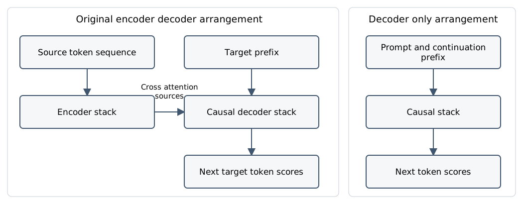
Original course diagram. Each stack contains multiple blocks; embeddings, normalization, and output details are omitted here.
The central components remain recognizable: learned token embeddings, residual states, attention, position-wise MLPs, and a vocabulary readout. Other choices vary independently. GPT-2 uses learned absolute position embeddings and pre-normalized blocks with LayerNorm. Its public implementation already includes past-key/value reuse. RoPE, RMSNorm, and grouped-query attention are not requirements for being a decoder-only Transformer. OpenAI GPT-2 implementation, pinned revision
Nor does the architecture alone establish conversational helpfulness, factual reliability, tool use, or a product’s permissions. Those also depend on training, input formatting, decoding, and the surrounding system.
Giving attention information about position
An attention operation with no positional signals and no order-dependent mask is permutation-equivariant: reorder the input rows, and its output rows reorder correspondingly. A causal mask already makes order relevant by changing which sources are available. Nevertheless, a model also benefits from explicitly representing where tokens occur and how far apart they are. Do not confuse the mask’s access restriction with a complete numerical encoding of distance.
The original paper adds fixed sinusoidal position vectors to token embeddings, and also evaluates learned position embeddings. GPT-2 adds a learned vector selected by the token’s absolute position. These additions preserve the residual width. Original Transformer, section 3.5
Rotary position embedding, usually shortened to RoPE, instead applies position-dependent rotations to query and key coordinates. Its basic construction makes their dot product depend on relative displacement through those rotations. It is not a rotation of tokens into geographical locations or a learned table of one vector for every possible position. Su et al., RoFormer, section 3
An exact two-coordinate rotation
For this calculation, use individual column vectors, unlike the row-stacked attention arrays in Lesson 2.2. Define
\[ R(\phi)=\begin{bmatrix} \cos\phi&-\sin\phi\\ \sin\phi&\cos\phi \end{bmatrix},\qquad \widetilde q_i=R(i\omega)q,\quad \widetilde k_j=R(j\omega)k. \]
Here \(R\) has shape \(2\times2\), and each vector has shape \(2\times1\). Choose the hand-constructed vectors
\[ q=\begin{bmatrix}2\\1\end{bmatrix},\quad k=\begin{bmatrix}1\\-1\end{bmatrix},\quad \omega=\pi/4. \]
This frequency makes the arithmetic exact and readable; it is not a claim about a particular checkpoint’s frequency schedule. Before rotation, \(q^{\mathsf T}k=1\).
Place the query at \(i=2\) and the key at \(j=0\). The query rotates by \(\pi/2\), while the key is unchanged:
\[ \widetilde q_2=\begin{bmatrix}-1\\2\end{bmatrix},\qquad \widetilde k_0=\begin{bmatrix}1\\-1\end{bmatrix},\qquad \widetilde q_2^{\mathsf T}\widetilde k_0=-3. \]
The lengths remain \(\sqrt5\) and \(\sqrt2\). Rotation changes relative direction without changing either vector’s norm. For a head of width two using the ordinary scaling, this pair contributes a score of \(-3/\sqrt2\) before masking and softmax. One score alone is not an attention probability.
Now shift both positions forward by one while holding the unrotated vectors fixed. At \(i=3,j=1\),
\[ \widetilde q_3=\begin{bmatrix}-3/\sqrt2\\1/\sqrt2\end{bmatrix},\qquad \widetilde k_1=\begin{bmatrix}\sqrt2\\0\end{bmatrix}. \]
Their dot product is still \(-3\). The general reason is
\[ \widetilde q_i^{\mathsf T}\widetilde k_j =q^{\mathsf T}R(i\omega)^{\mathsf T}R(j\omega)k =q^{\mathsf T}R((j-i)\omega)k. \]
The rotation term depends on \(j-i\). This identity does not say that moving an actual passage always leaves the model’s answer unchanged: its contextual representations and available sources can also change.
Extending the construction to a head
An even rotary width \(d_r\) contains \(d_r/2\) coordinate pairs. Each pair rotates at its own frequency. A basic schedule uses \(\omega_r=\theta^{-2r/d_r}\) for \(r=0,\ldots,d_r/2-1\). The head’s shape stays unchanged. Implementations can pair adjacent coordinates or corresponding coordinates from two halves; use the pairing expected by that implementation and checkpoint.
The rotary width need not always equal the full head width. Likewise, RoPE variants can rescale frequencies. In the Gemma specimen discussed here, the explicit head width is 256, and the reference implementation rotates query and key heads, leaving values unrotated. Different local and global frequency settings are part of its configuration. Google Gemma implementation
A formula can produce angles beyond a training sequence length. That mathematical fact does not establish reliable behavior at arbitrarily long contexts. Changing a frequency base or a context-limit field is not evidence that the model has learned to use the extended range.
A brief normalization checkpoint
Lesson 2.1 distinguished normalization type from its position in the block. LayerNorm subtracts the coordinate mean and divides by a stabilized standard deviation. RMSNorm divides by a stabilized root mean square without subtracting that mean:
\[ \operatorname{RMSNorm}(x)_a =\gamma_a\frac{x_a}{\sqrt{\frac1d\sum_bx_b^2+\epsilon}}. \]
This common expression includes learned scaling. Specific implementations can parameterize that scaling differently. Neither normalization is a mechanism for recognizing which facts are relevant. Zhang and Sennrich, RMSNorm
“Uses RMSNorm” does not tell you where every normalization occurs. Gemma 3 also uses query/key normalization and normalization on sublayer outputs. Read the actual addition boundaries before drawing its residual block. A pre-normalized branch, a normalized branch output, and normalization of the residual sum are different operations. Gemma 3 report, section 2
Query heads and KV heads need not have equal counts
Ordinary multi-head attention gives each query head its own key and value head. Multi-query attention, or MQA, shares one key head and one value head across all query heads. Grouped-query attention, or GQA, shares a KV pair within each group of query heads. MQA is the one-group endpoint; ordinary multi-head attention is the endpoint with one group per query head. Ainslie et al., section 2.2
Let \(h_q\) be the query-head count and \(h_{kv}\) the count of key heads, also the count of value heads. With eight query heads:
| Arrangement | \(h_q\) | \(h_{kv}\) | Query heads sharing each KV pair |
|---|---|---|---|
| Multi-head attention | 8 | 8 | 1 |
| Grouped-query attention | 8 | 2 | 4 |
| Multi-query attention | 8 | 1 | 8 |
Sharing keys does not force identical attention distributions. Two queries can score the same keys differently. Sharing values also does not force identical head outputs: different coefficients produce different mixtures.
Assume equal query, key, and value head width \(d_h\), residual width \(d\), and evenly sized groups. In the row-vector convention,
\[ \begin{aligned} W_Q&\in\mathbb R^{d\times(h_qd_h)},\\ W_K,W_V&\in\mathbb R^{d\times(h_{kv}d_h)},\\ W_O&\in\mathbb R^{(h_qd_h)\times d}. \end{aligned} \]
These are logical projections. An implementation may fuse Q, K, and V into one stored matrix or store matrix axes in the opposite order.
The KV projections become narrower when \(h_{kv}\) decreases. The query projections and number of query outputs need not shrink. Sharing changes representational capacity and storage; it is not merely a lossless file-compression setting. The original MQA work targets the memory traffic of incremental decoding. Real speed depends on the implementation and workload. Shazeer, Fast Transformer Decoding
Gemma 3 1B supplies a useful dimension check: \(d=1152\), \(h_q=4\), \(h_{kv}=1\), and \(d_h=256\). Thus its query projection outputs 1024 coordinates, its key projection 256, and its output projection maps 1024 back to 1152. Computing \(1152/4=288\) would give the wrong head width. The explicit configuration takes precedence over a familiar shortcut. This specimen is the MQA endpoint of the GQA family. Pinned Google configuration, get_config_for_1b
Reusing previous work with a KV cache
Suppose a causal model has processed a prompt at positions 0 through 99. To process a new token at position 100, its attention needs earlier keys and values. With fixed weights and unchanged prefix, correctly computed earlier states do not acquire information from the new token: causality prevents that backward dependency.
A KV cache retains earlier keys and values, separately for each attention layer. During prompt prefill, the engine computes the prompt’s states and populates the cache. During incremental decoding, it computes new states and reuses stored KV entries. It need not rerun the whole prefix through every layer for every new token. Transformers v4.51.3 caching explanation
Keep three different objects separate:
- \(W_K,W_V\): learned parameters shared across token positions;
- \(K,V\): activations calculated from a particular sequence;
- the cache: an inference data structure retaining those activations.
Adding a cache entry does not train the model. A different prompt generally needs different cached activations. Cache reuse also depends on the model, prefix, positions, masks, and computation being compatible. Editing an earlier token cannot safely leave all affected downstream prefix states untouched.
Past queries are usually unnecessary for ordinary next-token decoding: the current query reads past keys and values; old query results are not being recomputed. The new query still compares against permitted cached keys, so caching does not make global attention independent of context length.
Position bookkeeping matters. In RoPE implementations that store already-rotated keys, each cached key carries its original positional transformation. After processing 100 positions, the next logical position is 100, not zero. A rolling cache may overwrite a physical slot while logical positions continue increasing. Confusing slot number with logical position changes the computation. Padding and cache-position conventions are engine-specific; inspect both rather than copying a counter from a different API.
Context length and local attention describe different limits
A model’s context window is a stated supported sequence length, subject to its implementation and training. For ordinary autoregressive use, prompt tokens and generated tokens consume the available sequence budget together. Special tokens and other represented inputs may consume it too. A service can impose a smaller input or output cap.
A sliding attention window instead restricts which previous positions one layer can read directly. In a simple causal convention, a window of \(w\) includes the current position and at most \(w-1\) predecessors. Check whether a particular implementation counts the boundary the same way.
Local attention does not imply that all influence from older positions disappears after \(w\) tokens. A source representation can already contain information gathered by earlier layers. Multiple layers provide longer indirect paths, and a mixed architecture may also contain global layers. A possible path does not guarantee that a distant detail is retained or recovered accurately.
Gemma 3 interleaves five local layers and one global layer. Its 1B configuration specifies 26 layers, a 512-token local window, and 32,768 positions. Repeating that pattern gives four global layers and 22 local layers. The 1B variant is text-only; the larger family members’ vision support and 128K context should not be copied onto it. Gemma 3 report; pinned 1B configuration
The architecture and storage policy are separate. An engine can discard no-longer-needed local KV entries, but it can also allocate full-length arrays and merely mask the inaccessible positions. Google’s pinned reference generate implementation does the latter: it allocates the requested maximum sequence length in every layer. Therefore a local mask alone does not establish a small allocated cache. Reference allocation code
Turn cache dimensions into bytes
For conventional, uncompressed KV storage, assume:
- batch size \(B\), with the same stored length \(S\) per sequence;
- \(L\) layers, each with \(h_{kv}\) KV heads;
- key and value width \(d_h\);
- \(b\) bytes per stored scalar;
- no KV sharing between sequences, layers, or devices.
Each layer stores two arrays with logical shape \((B,h_{kv},S,d_h)\), regardless of physical axis order. Hence
\[ M_{KV}=2BLSh_{kv}d_hb\quad\text{bytes}. \]
The leading two counts keys and values. Use KV heads, not query heads. Kernels may temporarily expand shared KV heads for computation; that does not require the persistent cache to store those copies.
For the Gemma 1B dimensions, take \(B=1\), \(L=26\), \(S=32768\), \(h_{kv}=1\), \(d_h=256\), and \(b=2\). Full-length storage gives
\[ 2\cdot1\cdot26\cdot32768\cdot1\cdot256\cdot2 =872,415,232\text{ bytes}=0.8125\text{ GiB}. \]
Using four query heads in place of one KV head would overestimate this payload by a factor of four.
Now assume a different engine retains at most 512 entries in each local layer and the full prefix in each global layer. The steady-state retained payload becomes
\[ \begin{aligned} M_{KV} &=2Bh_{kv}d_hb\,[L_gS+L_\ell\min(S,w)]\\ &=1024\,[4\cdot32768+22\cdot512]\\ &=145,752,064\text{ bytes}\approx0.13574\text{ GiB}. \end{aligned} \]
This is an analytical estimate under the stated retention policy, not measured memory or the allocation of the reference generator. Chunked prefill, temporary tensors, alignment, reserved capacity, metadata, and device replication can change actual memory. Heterogeneous layers require summing their individual shapes. Doubling the independent batch doubles these payloads; it does not double the shared model weights.
Read configuration metadata without inventing runtime facts
Start by identifying the exact artifact and revision. This lesson uses GPT-2’s configuration snapshot and Google’s Gemma configuration factory. A factory contains defaults plus variant-specific overrides; it is not itself a trained checkpoint.
| Meaning | GPT-2 configuration | Gemma 3 1B factory |
|---|---|---|
| Residual width | n_embd: 768 |
hidden_size: 1152 |
| Block count | n_layer: 12 |
num_hidden_layers: 26 |
| Query heads | n_head: 12 |
num_attention_heads: 4 |
| KV heads | 12, established by implementation | num_key_value_heads: 1 |
| Head width | \(768/12=64\), established by implementation | head_dim: 256 |
| Position limit field | n_positions: 1024 |
max_position_embeddings: 32768 |
These references use different configuration schemas. The Hugging Face JSON uses vocab_size and n_positions; the historical OpenAI implementation uses n_vocab and n_ctx when constructing its embedding tables. We compare the architectural meanings, not claim that the JSON can be passed unchanged to that implementation. For this specimen the position-limit values agree at 1024.
A missing key is not permission to guess. Establish its default or interpretation from the matching model implementation. An intermediate_size describes an MLP width, not necessarily its parameter count: a gated MLP has more projections than a two-matrix MLP. Tied embedding/readout weights also affect parameter counting.
Likewise, dtype or torch_dtype metadata is not a measurement of every loaded tensor. Loading overrides, quantized modules, accumulators, and cache settings can differ. use_cache requests a behavior; it does not prove that a cache exists or occupies a particular amount of memory. A context-limit field does not certify long-context accuracy. Separate file facts, implementation facts, calculation assumptions, and runtime observations.
Lab 08 — Read Model Configurations and Estimate Memory turns the two specimens into an evidence table and a memory worksheet. Its core uses public text configurations and arithmetic only: no model weights, account, API, GPU, or paid compute.
Precision changes representation and memory
FP32 stores each scalar in four bytes. FP16 and BF16 each use two, but they allocate bits differently. BF16 has a wider exponent range than FP16 and fewer fraction bits. Equal storage size does not imply equal rounding behavior. Storage, multiplication, and accumulation can use different formats; a low-precision weight file does not establish the precision of every intermediate operation. Google Cloud’s BF16 explanation
Quantization represents values with a smaller set of possible levels. A simple affine scheme stores an integer \(q\) and reconstructs an approximation \(\hat x=s(q-z)\) using a scale \(s\) and zero point \(z\). For example, rounding \(x=1.1\) onto multiples of \(0.5\) gives \(q=2\) and \(\hat x=1.0\). The lost \(0.1\) does not return merely because the result is later represented in FP32.
Real methods differ in grouping, calibration, treatment of outliers, and which tensors remain at higher precision. Post-training quantization and quantization-aware training are different procedures. Quality effects must be evaluated for the model, method, and task; “four-bit” is not a complete accuracy specification. GPTQ paper
For an original weight-payload calculation, take exactly \(P=1,000,000,000\) stored scalar parameters. This is a round hypothetical count, not a claim that the name “1B” specifies an exact checkpoint count:
| Representation assumption | Payload bytes | Payload GiB |
|---|---|---|
| FP32, four bytes each | 4,000,000,000 | 3.72529 |
| FP16 or BF16, two bytes each | 2,000,000,000 | 1.86265 |
| Packed eight-bit values | 1,000,000,000 | 0.93132 |
| Packed four-bit values | 500,000,000 | 0.46566 |
For four-bit storage, \(P\times4/8=500,000,000\) bytes before overhead. Quantization scales, zero points or other metadata, unquantized tensors, and padding must be added. Weight quantization does not automatically quantize the KV cache. Transformers quantization documentation
An inference budget must also include cache, activations, temporary workspace, and runtime overhead. Training adds other large categories, including gradients and optimizer state. A weight-payload estimate is therefore not a promise that a machine of that capacity can run the model.
Smaller representations can reduce memory traffic, but conversion work, kernel support, hardware, batch size, and context length affect speed. Cache quantization can even increase latency in some conditions. Measure an explicitly defined workload rather than translating a fourfold storage reduction into a fourfold speedup. Transformers cache strategies
Check your understanding
- Does decoder-only imply RoPE, RMSNorm, or no processing of the prompt?
- In the rotation example, why did shifting both positions preserve the dot product? Would shifting only the query generally preserve it?
- A model has 16 query heads and four KV heads. How many query heads share each KV pair? Which count enters the persistent-cache formula?
- Does a 512-token local window imply a 512-token total context limit?
- What is missing from the claim “its weights take two GB, so it fits in two GB of memory”?
- A configuration says BF16. What further evidence would establish that the running cache is BF16?
- No. These are separate architectural choices, and the causal stack processes the prompt too.
- The displacement \(j-i\) stayed fixed while the unrotated vectors were held fixed. Moving only one position generally changes the relative rotation.
- Four queries per KV pair; four KV heads enter the cache formula.
- No. Local visibility is per layer; global layers or multi-layer paths can support longer dependencies. Actual supported length remains a separate question.
- Units, exact parameter count and storage format, cache, activations, workspace, overhead, and the workload. Quantized formats also require accounting for metadata and higher-precision tensors.
- Inspect the loaded cache tensors or the verified engine allocation path, including overrides. Configuration metadata alone is insufficient.
More Learning
- Attention Is All You Need — Vaswani et al. Revisit the two stacks and identify the cross-attention path removed in a conventional decoder-only design.
- RoFormer — Su et al. Read section 3.2 alongside the two-coordinate example; track the transpose and relative-position sign.
- GQA — Ainslie et al. Compare the MHA, GQA, and MQA head-sharing arrangements before reading performance claims.
- Root Mean Square Layer Normalization — Zhang and Sennrich Separate the normalization operation from where a model places it.
- Gemma 3 Technical Report Compare the family-level description with the linked 1B configuration. Preserve variant and memory-unit distinctions.
- Transformers caching explanation, v4.51.3 Trace prefill, incremental updates, attention masks, and logical positions. The pinned version is a concrete reference, not a recommendation to install it.
The next lesson examines Mixture of Experts, where selecting which MLP parameters participate in a token’s computation creates another distinction between total model size and active computation.