2.1 — The Residual Stream
Module 2 — The Transformer
Following a representation through depth
A Transformer repeatedly updates numerical representations of a sequence. The residual stream is a useful name for those representations as they pass through the network’s residual connections. Understanding this stream gives us a map: where a component receives its input, where it contributes an update, and what continues to the next component.
Lesson 1.2 introduced token embeddings and contextual representations. Lesson 1.3 opened a small neural network and distinguished parameters from activations. We now connect those ideas to a stack of Transformer blocks. We will leave the detailed attention calculation for Lesson 2.2 and the internal MLP computation for Lesson 2.3. Here, we need their interfaces and their places in the computation.
By the end, you should be able to:
- identify a token-position vector inside a sequence-shaped array;
- distinguish a branch’s update from the complete block output;
- trace residual additions and explain what their direct paths provide;
- recognize pre-norm, post-norm, and a parallel-residual variation;
- interpret vector changes without equating their size with knowledge or importance;
- specify exactly which activation an inspection tool should record.
Begin Reading the Original Transformer Paper, Part 1, before continuing. Read the abstract, introduction, architecture figure, and conclusion of Attention Is All You Need for orientation. Keep unfamiliar terms as questions. Return to the paper after Lesson 2.3; understanding every equation now is unnecessary.
Needed now: vector addition, matrix shapes, Euclidean norms, and affine transformations. The examples refresh these operations.
Useful refresh: a vector’s coordinates depend on a chosen basis; a dot product measures alignment with another vector.
Side trail: Jacobians and detailed optimization theory. One optional equation connects the residual path to the derivatives introduced in Lesson 1.3.
One vector per token position
Let a sequence contain \(n\) tokens, and let the model’s residual width be \(d\). At a chosen boundary in the network, collect its representations in
\[ X\in\mathbb{R}^{n\times d}. \]
Each row corresponds to a position, not to a unique vocabulary entry. Repeated token IDs still occupy separate rows. The number of coordinates in each row is the width \(d\), sometimes called hidden_size or \(d_{\mathrm{model}}\). It is independent of vocabulary size and sequence length.
We retain Lesson 1.3’s column convention when discussing one individual vector. For position \(i\), write \(x_i\in\mathbb{R}^{d}\) as a column, so row \(i\) of \(X\) is \(x_i^\mathsf{T}\). Thus the same information can be written
\[ X=\begin{bmatrix}x_1^\mathsf{T}\\x_2^\mathsf{T}\\\vdots\\x_n^\mathsf{T}\end{bmatrix}. \]
The transpose reconciles our two conventions. It does not perform a learned transformation. Software often adds a batch dimension, giving shape \((b,n,d)\) for \(b\) sequences; this chapter suppresses that dimension.
For an invented three-token sequence with width four, \(X\) contains twelve activation values. Adding another token adds another row. Passing through another width-preserving block produces another \(3\times4\) array. Neither operation adds vocabulary entries or automatically changes stored weights.
A row is not a separate little model for its token. After components exchange information between positions, that row can depend on a wider context. Conversely, the whole array is not one embedding vector for the entire conversation. Keeping both the position axis and the coordinate axis visible prevents these two pictures from being confused.
There are also two different orders to track. Position runs along the sequence; depth runs through blocks. A representation can change with depth while continuing to belong to the same position. Its eventual role in predicting a next token does not make it the embedding of that future token.
Where the stream starts
Token IDs select rows from the learned embedding matrix. For an architecture with additive positional embeddings, we can illustrate the initial representation as
\[ x_i^{(0)}=e_{t_i}+p_i, \]
where \(t_i\) is the token ID at position \(i\), \(e_{t_i}\) is its token embedding, and \(p_i\) carries positional information. Scaling and dropout may also occur, depending on the architecture and whether it is training or evaluating.
The original 2017 Transformer adds positional encodings to scaled token embeddings. Its full model has separate encoder and decoder stacks. This chapter instead uses a simplified decoder-only example, so its main diagram should not be read as a reproduction of the original architecture. Vaswani and colleagues, Sections 3.1, 3.4, and 3.5
Adding a position vector is not universal. In the Llama implementation referenced here, the stream starts from token embeddings, while rotary positional information acts on attention queries and keys. We will study that mechanism in Lesson 2.4. For now, remember that a model can use position without adding \(p_i\) to its initial stream. Transformers Llama implementation, v4.57.1
Two occurrences of the same ID retrieve the same token-embedding vector. Their later representations can differ because of position and available context. “The vector for a word” is therefore incomplete: ask which tokenizer, occurrence, checkpoint, depth, and measurement boundary.
A block computes updates and adds them
Start with the residual pattern
\[ y=x+F(x). \]
The residual branch computes \(F(x)\), and the skip connection carries \(x\) directly to the addition. The result \(y\) contains both numerical contributions. Addition requires matching shapes. A branch may use wider internal representations, but its output must return to the residual width before this addition.
The shape requirement creates a common interface. A branch may project into an internal space, do substantial computation there, and project back. It cannot append extra coordinates to the stream merely because it has found another useful pattern; that would change the shape required by the addition. Different contributions therefore coexist in the same finite-width representation. Their interaction can include reinforcement and cancellation.
A zero branch and an identity branch are also different. If \(F(x)=0\), the bare residual operation returns \(x\). If \(F(x)=x\), it returns \(2x\). When reading a diagram, label the branch output and the result of the addition separately rather than calling both of them “the residual.”
Residual learning predates the Transformer. He and colleagues used it to make very deep image-recognition networks easier to optimize. That history motivates the pattern; it does not make image models and language models identical. Deep Residual Learning for Image Recognition
For our main illustration, choose a sequential pre-norm decoder block, at evaluation time with dropout disabled. Let \(X^{(\ell)}\) enter block \(\ell\). Let \(N_{\ell,A}\) and \(N_{\ell,M}\) be its normalization operations. Define
\[ \begin{aligned} \Delta_A^{(\ell)}&=A_\ell\!\left(N_{\ell,A}(X^{(\ell)})\right),\\ Y^{(\ell)}&=X^{(\ell)}+\Delta_A^{(\ell)},\\ \Delta_M^{(\ell)}&=M_\ell\!\left(N_{\ell,M}(Y^{(\ell)})\right),\\ X^{(\ell+1)}&=Y^{(\ell)}+\Delta_M^{(\ell)}. \end{aligned} \]
\(A_\ell\) denotes attention, including its output projection; \(M_\ell\) denotes the MLP, including its projection back to width \(d\). Every displayed activation has shape \(n\times d\). Subscripts identify the block’s components, whose parameters are ordinarily different from those in other blocks.
The MLP receives a normalized version of the already attention-updated stream. It does not receive only the attention update. The block output is \(X^{(\ell+1)}\); calling \(\Delta_A^{(\ell)}\) or \(\Delta_M^{(\ell)}\) “the block output” would discard the skip-path contribution and confuse the boundary being measured. This sequential arrangement appears in the referenced Llama decoder implementation. Llama decoder block source
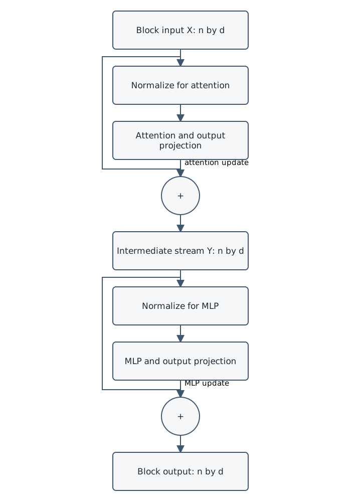
Original course diagram. One sequential pre-norm block; arrows describe dependencies rather than physical timing. Both direct arrows bypass a normalization-and-computation branch.
Prose alternative: The input splits into a direct path and an attention path. The attention path normalizes its input and calculates an update, which is added to the direct path. Their sum splits again. One copy goes directly to the second addition; the other is normalized and passed through the MLP. The second sum becomes the next block’s input.
An arrow in this diagram establishes a possible route for influence, not proof that a particular fact traveled along it. To establish an effect on an input, we must inspect values or perform a controlled comparison. A component can receive a vector while ignoring some directions in it, and a later component can counteract an earlier update.
Attention can use representations from other allowed positions to construct each position’s update. In a causal decoder, that means the current and permitted earlier positions, never later positions. A standard position-wise MLP transforms each position separately using shared parameters. Residual addition itself mixes neither positions nor coordinates: it adds matching entries. The branches supply the more complicated interactions.
An exact trace with three coordinates
We can isolate residual arithmetic without simulating attention. The following hand-constructed residual toy has no normalization, tokenizer, training, or claim to language understanding. Its two affine update functions are deliberately transparent:
\[ F(x)=\begin{bmatrix}-x_1\\2\\0\end{bmatrix}, \qquad G(y)=\begin{bmatrix}y_2\\-y_2\\2y_1\end{bmatrix}. \]
Here the subscripts select coordinates of one vector, rather than token positions. This local use is explicit to avoid confusing the two kinds of index. Let
\[ x=\begin{bmatrix}2\\-1\\1\end{bmatrix},\qquad y=x+F(x),\qquad z=y+G(y). \]
First calculate the branch output:
\[ F(x)=\begin{bmatrix}-2\\2\\0\end{bmatrix}. \]
Then add matching coordinates:
\[ y=\begin{bmatrix}2+(-2)\\-1+2\\1+0\end{bmatrix} =\begin{bmatrix}0\\1\\1\end{bmatrix}. \]
The next branch sees this new \(y\):
\[ G(y)=\begin{bmatrix}1\\-1\\0\end{bmatrix},\qquad z=\begin{bmatrix}1\\0\\1\end{bmatrix}. \]
We can check the same result by summing the input and the updates from this run:
\[ x+F(x)+G(y) =\begin{bmatrix}2\\-1\\1\end{bmatrix} +\begin{bmatrix}-2\\2\\0\end{bmatrix} +\begin{bmatrix}1\\-1\\0\end{bmatrix} =\begin{bmatrix}1\\0\\1\end{bmatrix}. \]
Notice cancellation. The first coordinate becomes zero after the first addition, even though the input arrived through an identity path. A residual connection does not promise to preserve each original value, or preserve every meaning we might associate with it.
The Euclidean norm measures vector length:
\[ \|x\|_2=\sqrt{\sum_jx_j^2}. \]
Our input has length \(\sqrt6\), and both \(y\) and \(z\) have length \(\sqrt2\). Equal lengths do not make \(y\) and \(z\) equal vectors. Nor must the stream’s norm grow when an update is added. Negative and differently directed contributions matter.
Now predict an intervention: suppress \(F(x)\), then recompute everything downstream. The second branch receives the original \(x\), giving \(G(x)=[-1,1,4]^\mathsf{T}\). The new output is \([1,0,5]^\mathsf{T}\). Merely subtracting the original \(F(x)\) from the original \(z\) would instead give \([3,-2,1]^\mathsf{T}\), which is wrong for this intervention. Later updates depend on what earlier components supplied.
In Trace a Residual Stream, make a fresh hand trace, compare update sizes with output effects, and explain an intervention. An optional second route records an actual small model’s states. Its measurements must come from an executed implementation; the toy numbers above are analytical examples.
What normalization changes
Normalization transforms the values a component receives or returns. It preserves the array’s shape while adjusting its numerical scale, and sometimes its centering. For the token-wise normalization considered here, the statistics are computed across the \(d\) coordinates of each position separately. They are not a mean across all tokens or all examples in a batch.
In a common LayerNorm form, first calculate a vector’s coordinate mean \(\mu\) and variance \(\sigma^2\). Then
\[ \operatorname{LN}(x)_j =\gamma_j\frac{x_j-\mu}{\sqrt{\sigma^2+\epsilon}}+\beta_j. \]
\(\epsilon>0\) stabilizes division; \(\gamma_j\) and \(\beta_j\) are learned scale and offset parameters when enabled. The standardized intermediate values are not themselves the final result when those learned parameters change them. PyTorch LayerNorm reference
RMSNorm uses the root mean square of the coordinates without first subtracting their mean. A common form is
\[ \operatorname{RMSNorm}(x)_j =\gamma_j\frac{x_j}{\sqrt{\frac1d\sum_kx_k^2+\epsilon}}. \]
The key distinction for this lesson is centering: RMSNorm does not perform LayerNorm’s mean subtraction. Details of learned parameters and numerical implementation still belong to the specific model. Zhang and Sennrich, Root Mean Square Layer Normalization; PyTorch RMSNorm reference
A small idealized comparison helps. For \(x=[1,3]^\mathsf{T}\), set scale to one, offset to zero, and temporarily ignore \(\epsilon\). LayerNorm gives \([-1,1]^\mathsf{T}\) because the mean is two and the variance is one. RMSNorm gives \([1/\sqrt5,3/\sqrt5]^\mathsf{T}\). Neither operation says which coordinate matters to the task. Normalization is a defined numerical transformation, not a filter that recognizes irrelevant meaning.
Pre-norm places normalization on a branch’s input:
\[ y=x+F(N(x)). \]
Post-norm normalizes after adding the branch output:
\[ y=N(x+F(x)). \]
These equations are different computations. In our pre-norm illustration, the direct stream bypasses the branch’s normalization. In the original Transformer’s post-norm sublayers, the summed result is normalized. Original Transformer, Section 3.1
Some modern designs combine additional normalization locations. Gemma 3’s report describes both pre- and post-normalization using RMSNorm. Do not force every model into one simplified diagram; inspect exactly what is normalized, and whether normalization occurs before or after the residual addition. Gemma 3 Technical Report, Section 2
Direct paths help optimization without guaranteeing preservation
Why carry the input directly? A residual branch can learn an adjustment to an existing representation rather than having to reproduce the entire representation through that branch. Setting the branch’s contribution to zero makes the bare residual operation an identity map. That offers a useful way to express small changes.
There is a corresponding derivative intuition. For the simplified equation \(y=x+F(x)\),
\[ \frac{\partial y}{\partial x}=I+J_F(x), \]
where \(I\) is the identity matrix and \(J_F\) collects the local sensitivities of \(F\). The direct term provides a gradient path in addition to the transformed path. Identity-path analysis is a central theme of subsequent residual-network research. He and colleagues, Identity Mappings in Deep Residual Networks
This does not guarantee nonvanishing gradients. If \(F(x)=-x\), then \(y=0\) and \(I+J_F=0\). The same counterexample defeats a claim that residual addition must preserve recoverable input information. An available route in the computation graph is different from a mathematical guarantee about the complete function.
Placement of normalization also changes gradient behavior. Research comparing pre-norm and post-norm Transformers analyzes how their gradient scales differ at initialization and why training procedures can behave differently. The practical outcome depends on the complete architecture, initialization, and optimization setup. “Residuals solve training” is too strong. Xiong and colleagues, 2020
For our sequential pre-norm stack, algebra in exact arithmetic lets us write its final raw stream as its initial stream plus all residual updates along the actual forward pass:
\[ X^{(L)}=X^{(0)}+ \sum_{\ell=0}^{L-1}\left(\Delta_A^{(\ell)}+\Delta_M^{(\ell)}\right). \]
This is accounting, not a claim that the updates are independent. Each was calculated using preceding states. Nor does the same expression automatically describe the normalized boundaries of a post-norm stack. Keep the equation attached to the architecture for which it was derived.
Accumulation is not a readable list of facts
The stream can carry information useful to many later operations, but its coordinates are not text fields with stable human labels. An update might reinforce a direction, counteract an earlier contribution, or rearrange what later transformations can use. “More layers accumulate more knowledge” hides these possibilities and confuses activations with learned parameters.
Consider a downstream scalar readout \(s=w^\mathsf{T}x\). An update \(\delta\) changes that immediate readout by \(w^\mathsf{T}\delta\). Its norm alone cannot determine the change. A large update perpendicular to \(w\) has zero effect on this particular readout; a smaller aligned update can matter. In a full model, later nonlinear computations complicate the relationship further.
Coordinate labels also depend on the representation’s basis. Swapping two coordinates and consistently swapping the corresponding parameters can preserve a compatible computation. Orthogonal changes of coordinates preserve Euclidean lengths and angles; arbitrary invertible changes generally do not. Do not conclude that every basis change preserves a complete Transformer without adjusting or respecting its normalization and other architectural constraints.
Within one checkpoint’s residual space, comparing vectors at stated boundaries can be useful. Across separately trained models, coordinate 17 is not automatically the same feature. Even within one model, cosine similarity or distance is a numerical observation that needs a task-specific interpretation. A heatmap does not supply that interpretation by itself.
Finally, depth is not lasting memory. Ordinary inference computes fresh activations using fixed parameters. Runtimes may cache intermediate quantities for efficient generation, but a changed residual state is not evidence that the model has learned new weights or permanently stored the conversation.
Inspect the actual boundary
An inspection must name the checkpoint, input tokens, token position, block, and location relative to normalization and addition. A field called hidden_states is an interface choice; it does not universally mean every raw post-addition state. A final normalization can make the last returned state different from the last block’s raw output.
There are topology differences too. The optional Lab uses Pythia-14M, whose pinned configuration selects parallel residuals. In that arrangement, attention and MLP read separately normalized versions of the same block input:
\[ X^{(\ell+1)}=X^{(\ell)}+ A_\ell(N_{\ell,A}(X^{(\ell)}))+ M_\ell(N_{\ell,M}(X^{(\ell)})). \]
The MLP does not read the attention-updated state inside that block. The checkpoint has six blocks and residual width 128. Its small scale is convenient for inspection, but its topology must not be silently relabeled as our sequential example. Pinned Pythia configuration; GPT-NeoX layer implementation
After a decoder stack, a final normalization and vocabulary projection may convert the stream into logits. In row-array notation, if \(H=N_f(X^{(L)})\) and \(W_U\) has shape \(d\times V\), then \(HW_U\) has shape \(n\times V\). An optional vocabulary bias is broadcast across positions. Residual width and vocabulary size play different roles all the way to the output.
We now have the surrounding structure. Next, attention will explain how one position computes a context-dependent update from allowed positions. The residual addition tells us where that update goes; attention tells us how it is calculated.
Check your understanding
- A batch contains two sequences of nine tokens, with residual width 128. What is its activation shape? Does six blocks imply a width of \(6\cdot128\)?
- In the sequential pre-norm equations, what does the MLP read? What changes in the parallel arrangement?
- If a branch update is zero, when is the operation necessarily the identity: \(x+F(N(x))\), or \(N(x+F(x))\)?
- Why can a later stream have a smaller norm than an earlier stream?
- Why was subtracting the original first update insufficient to predict our toy intervention?
- What evidence is missing from “this layer changed the vector most, so it did the most reasoning”?
- Shape \((2,9,128)\). Six width-preserving blocks change depth, not width; each boundary retains that shape.
- It reads \(N_{\ell,M}(Y^{(\ell)})\), the normalized attention-updated state. In the parallel arrangement it reads its own normalized version of the block input.
- Zeroing the pre-norm branch gives \(x\). Zeroing the post-norm branch gives \(N(x)\), which need not equal \(x\).
- Updates can oppose existing coordinates or directions. Normalization can also change scale, so measurement boundaries matter.
- The intervention changed the second branch’s input. Its output had to be recomputed rather than held at its baseline value.
- Vector distance measures numerical change at a boundary. A reasoning claim requires a defined behavior, appropriate comparisons, and evidence connecting that change to the behavior, ideally including controlled interventions.
More Learning
- Attention Is All You Need. Use the staged reading Lab. For this chapter, identify residual additions and normalization in Section 3.1; save attention’s equations for the next lesson.
- Deep Residual Learning for Image Recognition and Identity Mappings in Deep Residual Networks. Historical primary sources for residual learning and direct paths. Their computer-vision experiments are not measurements of LLM behavior.
- Layer Normalization and Root Mean Square Layer Normalization. Read the definitions first. Derive the two-coordinate example before attempting the training analyses.
- On Layer Normalization in the Transformer Architecture. An optional mathematical treatment of normalization placement and optimization. Separate the paper’s analyzed setting from universal claims.
- Gemma 3 Technical Report. A contemporary architecture comparison. Mark details that our simplified diagram omits; Lesson 2.4 will make more of them familiar.
- Pythia-14M model card. Read the intended use and limitations before the optional model-inspection Lab. Small and inspectable does not imply suitable for deployment.