1.3 — Neural Networks Without the Mysticism
Module 1 — Foundations: From AI to LLMs
A network you can account for
A neural network takes numbers, transforms them through a sequence of operations, and produces more numbers. Its learned parameters determine many details of those transformations. That description sounds ordinary because the individual operations usually are. The difficulty comes from how many operations interact, how training selects their parameters, and how we establish what the resulting system does.
In Lesson 1.2, we followed text into numerical representations and model outputs back toward text. Here we open the computation between those endpoints. We will use two input numbers, three hidden units, and one numerical output. Every intermediate value will fit on a page. The example is deliberately hand-constructed; nobody trained it, and it has no claimed real-world predictive ability.
By the end, you should be able to:
- read a small network equation and check its dimensions;
- distinguish weights, biases, activations, and architecture choices;
- compute a forward pass and predict a controlled intervention;
- explain why nonlinear operations matter;
- separate inference, gradient calculation, and parameter updates;
- describe what a successful calculation does, and does not, establish.
The same habits will help when a Transformer replaces our three hidden units with much larger computations.
Needed now: multiplying and adding signed numbers; vectors; dot products; matrix multiplication; functions; a derivative as local sensitivity. We develop each operation below.
Useful refresh: rows versus columns, transposes, coordinates, and the difference between a scalar and a vector.
Side trail: Jacobians, rank, formal approximation theorems, and optimization theory. They offer deeper explanations but are unnecessary for the forward pass. The Lab includes an optional one-parameter derivative check.
Numbers with roles and shapes
A scalar is one number. A vector is an ordered collection of numbers. A matrix is a rectangular arrangement of numbers. For this lesson, individual vectors are columns:
\[ x=\begin{bmatrix}2\\-1\end{bmatrix}. \]
The notation \(x\in\mathbb{R}^2\) says that \(x\) has two real-valued coordinates. Its column-array shape is \(2\times1\). An implementation may instead store a one-dimensional array with shape (2,); we must specify the convention before multiplying it.
The coordinates could be two measured features, two intermediate values, or two deliberately invented inputs. The arithmetic does not tell us their real-world meaning. If they represented temperature and distance, their units and scaling would also matter. For this example they are simply dimensionless numbers.
A dot product multiplies corresponding coordinates and adds the results. With weights \(w=[1,-1]\), the dot product with our input is
\[ w\cdot x=(1)(2)+(-1)(-1)=3. \]
Notice the negative input and negative weight: their contribution is positive. A weight’s sign is not a label saying that a feature is good or bad. It specifies a numerical relationship in a particular computation.
A matrix lets us compute several weighted sums at once. Put one set of weights in each row:
\[ W=\begin{bmatrix} 1&-1\\ 0.5&1\\ -1&2 \end{bmatrix}. \]
There are three rows and two columns, so \(W\) has shape \(3\times2\). Multiplying \(Wx\) takes a dot product between each row and the same input. Three rows produce three outputs. The inner dimensions must agree:
\[ (3\times2)(2\times1)=(3\times1). \]
This is the first useful debugging habit: write shapes beside the equation before calculating values. A \(3\times2\) matrix cannot multiply a \(4\times1\) column in this way. An extra or missing dimension often signals that we have mixed up examples, features, or sequence positions.
Weights and biases define an affine layer
For one unit, a weighted sum plus a bias is
\[ z_j=\sum_{i=1}^{2}W_{ji}x_i+b_j. \]
The index \(i\) selects an input coordinate; \(j\) selects an output unit. The bias contributes even when every input is zero. Collecting all three units gives
\[ z=Wx+b,\qquad b=\begin{bmatrix}0\\1\\0.5\end{bmatrix}. \]
Here \(z\) is the preactivation: the value before the activation function we will apply next. The vectors \(z\) and \(b\) both have three coordinates. Addition happens coordinate by coordinate.
Strictly, \(Wx\) is a linear transformation. Adding a nonzero bias makes \(Wx+b\) affine. A linear map sends zero to zero; an affine map may shift it elsewhere. Machine-learning libraries commonly use the name “linear layer” for this affine operation. PyTorch’s Linear, for example, includes an optional learned bias and documents its weight shape as output features by input features. Its row-oriented input convention is equivalent to ours after transposing the vectors. PyTorch Linear documentation
Each row forms a weighted combination of the input coordinates. The bias shifts the resulting value. For our first unit, \(z_1=x_1-x_2\). Inputs with \(x_1=x_2\) give zero. Changing its bias to \(1\) would move the zero boundary to \(x_1-x_2=-1\).
For a dense affine layer with \(d\) inputs and \(m\) outputs, there are \(md\) weights and, if enabled, \(m\) biases. Our first layer therefore contains \(3\cdot2+3=9\) parameters. That count describes stored adjustable numbers, not nine facts or nine concepts.
Activation functions change what composition can express
We now apply the rectified linear unit, or ReLU, separately to each coordinate:
\[ h_j=\operatorname{ReLU}(z_j)=\max(0,z_j). \]
Positive values pass through unchanged; negative values become zero. ReLU preserves the vector’s shape. We call \(h\) the hidden activation vector. “Activation” can refer either to the function, such as ReLU, or to a computed value, such as \(h_2=1\). Context should make the meaning clear. PyTorch ReLU documentation
Why add this operation? Consider two affine layers with nothing nonlinear between them:
\[ u=Ax+a,\qquad y=Bu+b. \]
Substitution gives
\[ y=B(Ax+a)+b=(BA)x+(Ba+b). \]
The whole composition is another affine transformation. Its factorization can matter for parameterization and optimization, but stacking these layers has not introduced a nonlinear input-output function.
ReLU breaks that general simplification. For an immediate counterexample, \(\operatorname{ReLU}(1)+\operatorname{ReLU}(-1)=1\), while \(\operatorname{ReLU}(1+(-1))=0\). It does not preserve addition, one requirement of linearity.
Within a region where the same ReLU units remain positive, our network will still have an affine formula. Crossing a zero boundary can change that formula. The resulting function is piecewise affine, often called piecewise linear in neural-network discussions. Nonlinearity gives the architecture additional possibilities; particular weights can still produce a constant or affine function.
Other activation functions make different trade-offs. A nonlinear function need not clip negative values, and ReLU is not a requirement for every network. We use it because its behavior is easy to inspect by hand. Later MLP lessons will revisit the choices used inside language models.
If a hidden unit’s preactivation is negative, will increasing its output weight change this example’s prediction? Write down your answer and the condition on which it depends. We will test exactly this question.
The complete microscopic network
Our output is one unconstrained real number, suitable as the form of a regression prediction. We use a final affine readout without another ReLU:
\[ h=\operatorname{ReLU}(Wx+b),\qquad \hat y=v^\mathsf{T}h+c, \]
where
\[ v=\begin{bmatrix}2\\-1\\1\end{bmatrix},\qquad c=0.5. \]
The hat in \(\hat y\) marks a prediction. It does not mean that the prediction is accurate. The final row \(v^\mathsf{T}\) has shape \(1\times3\), so its product with \(h\) is a scalar. A classification model could instead have several output scores, or logits, followed by the interpretation discussed in Lesson 1.2. We keep one output to concentrate on the network itself.
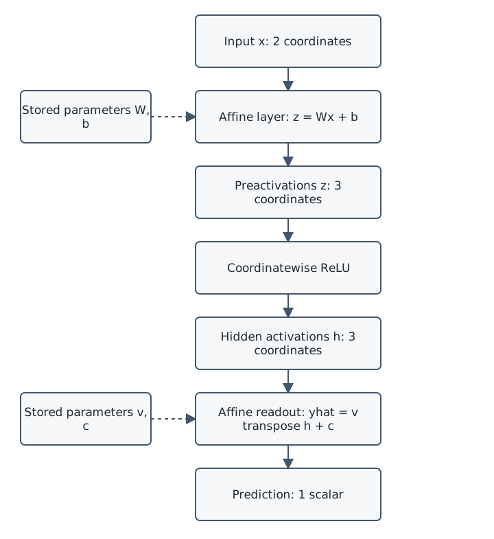
Original course diagram. Read downward along the solid arrows: two inputs become three preactivations, then three ReLU activations, then one prediction. The dotted arrows show which stored parameters each affine operation reads. Applying this graph does not itself change those parameters.
A network of this form is a small feedforward network or multilayer perceptron: intermediate computations depend on earlier ones in the forward graph. Its hidden layer is “hidden” because the task supplies inputs and desired outputs rather than a target value for every intermediate unit. The values are still observable when we instrument the computation. Goodfellow, Bengio, and Courville, Chapter 6
People count layers differently. This example has one hidden layer and one output layer, both parameterized. ReLU may be a separate software module. “Two-layer network” without a counting convention is less informative than the equations.
Compute every intermediate value
Start with \(x=[2,-1]^\mathsf{T}\). Before reading the answers, calculate all three entries of \(z\).
\[ \begin{aligned} z_1&=(1)(2)+(-1)(-1)+0=3,\\ z_2&=(0.5)(2)+(1)(-1)+1=1,\\ z_3&=(-1)(2)+(2)(-1)+0.5=-3.5. \end{aligned} \]
Thus
\[ z=\begin{bmatrix}3\\1\\-3.5\end{bmatrix}, \qquad h=\begin{bmatrix}3\\1\\0\end{bmatrix}. \]
The readout is
\[ \hat y=(2)(3)+(-1)(1)+(1)(0)+0.5=5.5. \]
Three details matter. First, the negative preactivation was removed before the readout. Second, the positive activation \(h_2=1\) contributes negatively because its readout weight is \(-1\). Third, the output bias is added once. It is not added separately to every contribution.
The full parameter count is \(6+3+3+1=13\): six entries in \(W\), three in \(b\), three in \(v\), and one in \(c\). The intermediate vectors are additional values computed for this input, not additional learned parameters.
Intervene and explain the difference
Hold the input and parameters fixed, but replace \(h_2\) with zero immediately before the readout. This ablation produces
\[ \hat y_{\mathrm{ablated}}=(2)(3)+(-1)(0)+(1)(0)+0.5=6.5. \]
Removing a unit’s contribution increased the output. Its original contribution was \(-1\). “More activation means more output” is therefore an unsafe general rule even in this tiny network.
Now restore the original activations and change only \(v_3\) from \(1\) to \(101\). The output remains \(5.5\), since \(h_3=0\). This answers the prediction question for this input. On another input, the same parameter can matter substantially. With \(x=[0,1]^\mathsf{T}\), calculate \(z=[-1,2,2.5]^\mathsf{T}\) and \(h=[0,2,2.5]^\mathsf{T}\). The original output is \(1\); changing \(v_3\) to \(101\) makes it \(251\).
A zero intervention effect on one example therefore does not establish global irrelevance. Conversely, a nonzero effect establishes a dependency in the tested computation; by itself it does not assign the unit a human concept.
Do Tiny Network, Visible Computation, Parts 1–3. Compute a fresh forward pass by hand before implementing it, then predict an intervention before running it. The core Lab needs only paper and, optionally, ordinary Python on a CPU. No account, API, model download, or paid compute is needed.
Parameters persist while activations change
Write the network as \(f_\theta(x)\), where \(\theta\) collects \(W,b,v,c\). This notation separates the input from the stored numbers defining the particular function.
In ordinary inference, we apply a chosen parameter set to an input. Changing \(x\) generally changes \(z\), \(h\), and \(\hat y\). It need not change \(\theta\). In our deterministic example, the same input and same parameters give the same output. Larger systems may add sampling or other sources of variation.
In training, a procedure updates selected parameters to improve an objective on training examples. Parameters can be trainable in that procedure or frozen, meaning that procedure leaves them unchanged. A frozen weight still participates in the forward calculation and affects its output. If we freeze \(W\) and \(b\), our model still stores 13 parameters, but only the four numbers in \(v\) and \(c\) remain candidates for updates.
Architecture choices sit at another level: this network’s hidden width is three, its hidden function is ReLU, and its output is scalar. Ordinary gradient updates to the 13 numbers do not decide to add another hidden unit. Likewise, a learning rate controls an update procedure rather than appearing as a learned coefficient in this forward equation.
A new conversation message can change a language model’s input and activations without an update to its stored weights. Whether a particular service separately uses conversations for later training is a product and data-policy question. The forward computation alone does not answer it.
If \(B\) examples are stored as rows in \(X\) with shape \(B\times2\), the equivalent first-layer calculation is \(Z=XW^\mathsf{T}+\mathbf{1}_B b^\mathsf{T}\), where \(\mathbf{1}_B\) is a column of \(B\) ones. This adds the same bias row to every example. In code, a one-dimensional length-three bias array can be broadcast across those rows. Then \(Z\) and \(H\) have shape \(B\times3\), and \(Hv+c\) produces one output per example. The transpose accommodates storage orientation; it does not change the network. PyTorch’s Linear specification is a useful reference when checking this convention.
Dimension agreement is necessary but insufficient. Swapping two feature columns preserves the shape while changing their meaning. Track both the size and the role of each axis.
Training adds an objective and an update
Suppose one training example asks for target \(t=4\) at our original input. Choose a loss
\[ L=\tfrac12(\hat y-t)^2. \]
At \(\hat y=5.5\), the error is \(1.5\) and the loss is \(1.125\). The factor \(\tfrac12\) makes the derivative convenient. This is a chosen instructional objective, not a claim that squared error is appropriate for every task.
A basic training step performs a forward pass, computes loss, calculates gradients, and uses an optimizer to update selected parameters. Backpropagation calculates the gradients; an optimizer uses them to update parameters. Merely calculating a gradient does not change a weight. PyTorch exposes this distinction through separate backward and optimizer operations. PyTorch optimization tutorial
A derivative answers a local sensitivity question. If we change one parameter slightly while holding the others fixed, how quickly does the loss change? For \(v_1\), the path to the loss is short:
\[ \frac{\partial L}{\partial\hat y}=\hat y-t=1.5, \qquad \frac{\partial\hat y}{\partial v_1}=h_1=3. \]
The chain rule multiplies sensitivities along this path:
\[ \frac{\partial L}{\partial v_1} =\frac{\partial L}{\partial\hat y} \frac{\partial\hat y}{\partial v_1} =1.5\cdot3=4.5. \]
The positive sign says that a sufficiently small increase in \(v_1\) raises this loss locally. A gradient-descent update with learning rate \(\eta=0.1\), changing only \(v_1\), gives
\[ v_1^{\mathrm{new}}=2-0.1(4.5)=1.55. \]
The new prediction is \(1.55(3)-1+0.5=4.15\), giving loss \(0.01125\). These are exact hand-derived values for this chosen example. We have fitted one parameter toward one target; we have not demonstrated a useful trained model.
For an earlier weight, the sensitivity passes through more operations. Since \(z_1=3\) is positive, ReLU has slope one there:
\[ \frac{\partial L}{\partial W_{11}} =(\hat y-t)\,v_1\,(1)\,x_1 =1.5\cdot2\cdot1\cdot2=6. \]
This derivative uses the original parameters. ReLU’s slope is zero on a strictly negative input, and its ordinary derivative is undefined exactly at zero; implementations choose a convention there. Automatic differentiation applies such local rules through a recorded computation graph. It saves us from hand-expanding a large network. PyTorch automatic differentiation tutorial
A gradient is local information. A large step can overshoot, an update that helps one example can hurt another, and a training objective may only imperfectly represent the behavior we ultimately want. Module 3 will develop training across datasets and repeated updates.
What the neuron metaphor leaves out
In this MLP, a “neuron” usually means one hidden coordinate together with its incoming weighted sum and activation function. The term does not establish that it models the detailed biology of a nerve cell. We can specify every operation here without claims about thoughts, intentions, or experience.
Nor should we assume that each coordinate has a stable, human-readable meaning. A single activation may participate in several patterns, and an interpretable property may involve several coordinates. Research on superposition explores how networks can represent more features than their representation has dimensions. Toy Models of Superposition demonstrates mechanisms in deliberately simplified models; its results motivate questions about larger networks rather than automatically settling them. We will return to this in Lesson 2.3. Elhage and colleagues, 2022
Even our example discourages quick labels. Unit 3 is inactive for one input and important for another. Unit 2’s positive activation lowers the scalar readout. Naming either unit from one observation would lose crucial conditions. A useful interpretation must say which inputs it covers, which computation it describes, and what evidence could contradict it.
Evaluation asks a different question
Getting \(5.5\) proves that a particular forward calculation matches the specified arithmetic. Passing the Lab’s checks can establish that an implementation matches that specification. Neither result establishes predictive accuracy on a real task.
For a trained model, examine performance on examples not used to fit its parameters. Use validation data for development decisions and protect a separate test set for final evaluation. Data leakage can happen through preprocessing and model selection as well as direct training. Scikit-learn’s guidance on data leakage
For this network, useful evaluation would first require a defined task: what do the two inputs mean, what target should the output approximate, and which mistakes matter? Only then could we choose appropriate data and measurements. A falling training loss answers one optimization question. It does not establish robustness, calibration, fairness, or suitability for a particular use.
There is also a boundary between tracing and explaining. We can trace every multiplication and still need an explanation of why this function fits a task. At larger scales, recording activations is a starting point for investigation. It is not automatically a readable account of what the model represents.
The bridge to Transformers
The original Transformer contains position-wise feedforward networks with two affine transformations and a ReLU between them. That component is a close relative of the computation we have just inspected. The architecture also includes attention and residual connections, which give the larger system additional structure. Vaswani and colleagues, Section 3.3
Carry forward three questions: What shape enters this operation? Which stored parameters does it use? What new activation does it produce? They remain useful when the numbers no longer fit on a page. The next module will add the residual stream and show how multiple components read and update token representations.
Check your understanding
Answer without looking back, then compare with the solutions.
- Why are \(Wx+b\) and \(\operatorname{ReLU}(Wx+b)\) generally different kinds of functions?
- For \(x=[1,0]^\mathsf{T}\), compute \(z\), \(h\), and \(\hat y\) using the original parameters.
- Remove ReLU from the original network. Find its simplified input-output equation and its output at \([2,-1]^\mathsf{T}\).
- A unit’s ablation has no effect on one input. What can you conclude? What extra claim is unjustified?
- Which changes an activation: changing the input, updating a weight, or both? Which necessarily updates a stored parameter?
- Why does a correct implementation still need evaluation on a task?
- The first is affine. ReLU can change which coordinates pass through as inputs change, allowing a piecewise-affine function. Particular parameters can still make the full function affine.
- \(z=[1,1.5,-0.5]^\mathsf{T}\); \(h=[1,1.5,0]^\mathsf{T}\); \(\hat y=2-1.5+0.5=1\).
- \(v^\mathsf{T}W=[0.5,-1]\) and \(v^\mathsf{T}b+c=0\). Thus \(\hat y=0.5x_1-x_2\), giving \(2\). The original ReLU network gives \(5.5\) there.
- Only that this intervention had no measured effect under the tested conditions. The unit need not be irrelevant for other inputs or other readouts.
- Both can change activations, though neither guarantees a change at every coordinate. Updating a weight changes a stored parameter; changing the input alone does not.
- Correctness against a specification establishes that we computed the intended function. Task evaluation tests whether that function gives useful outputs under relevant conditions.
More Learning
- Goodfellow, Bengio, and Courville: Deep Feedforward Networks. Read the opening definitions and Section 6.5 for a more formal treatment of composition and backpropagation. The chapter is broader than this lesson; treat the later details as optional.
- PyTorch Linear and ReLU. Short official references for the two operations. Compare their input, output, and parameter shapes with our equations before using a library implementation.
- PyTorch: Automatic Differentiation. Connect the hand-calculated chain rule to a computational graph and stored gradients. No PyTorch installation is required to read it.
- PyTorch: Optimizing Model Parameters. Follow the separation of loss calculation, backward calculation, and optimizer updates. Its larger training example is optional; the nearby course Lab stays microscopic.
- Elhage and colleagues: Toy Models of Superposition. An advanced preview of why a neuron and an interpretable feature are different objects. Focus initially on the abstract and the limits of conclusions from toy models.
- Vaswani and colleagues: Attention Is All You Need. Read Section 3.3 and recognize the affine–activation–affine pattern. Save the full architecture for Module 2.