2.2 — Attention
Module 2 — The Transformer
How one position reads another
The residual stream gives each token position a working vector. Attention lets a position construct an update using vectors at other permitted positions. The update depends on both the current representations and learned parameters. Following that computation will help us understand how context changes a model’s behavior without changing its stored weights.
Consider the unfinished sentence “The key beside the cabinets …”. Predicting what follows may require information from several earlier positions. A model could use attention to bring information about “key” toward the position producing the prediction. That is a possible computation to investigate, not a claim that an unspecified model contains a dedicated grammar head. Real token boundaries may also differ from the word boundaries in this illustration.
We will build one attention head small enough to calculate exactly, then connect it to multi-head attention and the residual stream. We will also establish a careful limit: an attention map exposes one intermediate computation, but cannot by itself explain the model’s final answer.
By the end, you should be able to:
- distinguish query, key, and value vectors from their learned projection matrices;
- check the dimensions of an attention calculation;
- compute scaled scores, masked row-wise softmax, and a weighted value mixture;
- explain which information a causal position may access;
- describe how several heads produce a residual-stream update;
- evaluate a claim made from an attention visualization.
The prerequisite is Lesson 2.1 — The Residual Stream. Keep its distinction between a residual state and a sublayer’s contribution in view.
Needed now: dot products, matrix multiplication, transpose, exponentials, and normalization by a sum. We use these operations explicitly below.
Useful refresh: the softmax from Lesson 1.2, row versus column conventions from Lesson 1.3, and the fact that a dot product depends on both direction and magnitude.
Side trail: variance calculations behind the scaling factor, derivatives through softmax, and matrix rank. None is required to complete the worked example.
Three projections of the same input
For this lesson, stack the vectors supplied to attention as rows:
\[ X\in\mathbb{R}^{n\times d_{\text{model}}}. \]
There are \(n\) token positions and \(d_{\text{model}}\) coordinates per position. Lesson 1.3 initially used individual column vectors. Here \(x_i\) is a row, so we multiply a projection matrix on its right. Transposing both representations recovers the other convention; the underlying operation is unchanged.
\(X\) means the input actually supplied to this attention sublayer. In a pre-normalized block, it is the normalized residual state. It need not be the original token embedding, and we should not silently replace it with one.
One head forms three arrays:
\[ Q=XW_Q,\qquad K=XW_K,\qquad V=XW_V. \]
Their roles differ:
- A query \(q_i\) is used by destination position \(i\) to score possible sources.
- A key \(k_j\) is the vector against which source position \(j\) is scored.
- A value \(v_j\) is the vector mixed into the destination’s result.
The names suggest a lookup, but the computation usually returns a mixture of values rather than one selected record. Queries are numerical vectors, not textual questions; keys are numerical vectors, not labels identifying concepts.
If queries and keys have \(d_k\) coordinates and values have \(d_v\) coordinates, then
\[ \begin{aligned} W_Q,W_K&\in\mathbb{R}^{d_{\text{model}}\times d_k}, &Q,K&\in\mathbb{R}^{n\times d_k},\\ W_V&\in\mathbb{R}^{d_{\text{model}}\times d_v}, &V&\in\mathbb{R}^{n\times d_v}. \end{aligned} \]
The query and key widths must match because we take their dot product. The value width can differ. Within this head, the same \(W_Q\), \(W_K\), and \(W_V\) apply at every position. Their entries are learned parameters; the entries of \(Q\), \(K\), and \(V\) are computed activations. We omit optional projection biases to keep the equations readable.
These equations are the standard projected attention construction introduced in the original Transformer. The distinction between the three projections is important: a source’s compatibility score and the content it contributes are calculated through different matrices. Vaswani et al., section 3.2
Scores become a distribution over sources
Form the scaled score matrix
\[ S=\frac{QK^{\mathsf T}}{\sqrt{d_k}},\qquad S_{ij}=\frac{q_i\cdot k_j}{\sqrt{d_k}}. \]
The product has shape \((n\times d_k)(d_k\times n)=n\times n\). Rows identify destinations; columns identify sources. Entry \(S_{ij}\) is a score for destination \(i\) reading source \(j\). Transposing the map reverses those roles.
A score is neither a probability nor a measured semantic similarity. Learned projections determine which input directions contribute to the dot product. Increasing a vector’s magnitude can change the score without changing its direction, so ordinary dot-product attention is not cosine similarity.
The divisor uses the query/key width \(d_k\), not the number of positions and not automatically the residual width. The original paper motivates it with an idealized calculation: independent, zero-mean, unit-variance query and key coordinates give a dot product with variance \(d_k\). Dividing by \(\sqrt{d_k}\) counters that growth. Trained activations need not satisfy those assumptions; the scaling is not a guarantee that all scores have a particular distribution. Vaswani et al., section 3.2.1
We then apply softmax across the source columns of each row. For an allowed-source set \(J_i\),
\[ A_{ij}=\frac{\exp(S_{ij})}{\sum_{r\in J_i}\exp(S_{ir})} \quad\text{when }j\in J_i, \]
and \(A_{ij}=0\) otherwise. Here we inspect weights with attention-weight dropout disabled. Each valid row sums to one. The columns need not sum to one: several destinations can read the same source strongly. Attention does not allocate an exclusive supply of information that other positions then lose.
These weights resemble the probabilities from Lesson 1.2, but their axis and role differ. A vocabulary softmax produces weights over possible output tokens. This softmax produces mixture coefficients over permitted source positions. No token is sampled here.
For numerical stability, software can subtract the largest allowed score in a row before exponentiating. The common factor cancels between numerator and denominator. For example, \([1000,1000]\) and \([0,0]\) both yield \([1/2,1/2]\), while the latter avoids computing enormous exponentials.
If all allowed scores in a row are equal, what weights result? If one score remains unchanged but a competing score increases, does the first source retain its old weight? Explain using the denominator.
A mask defines the available information
For causal self-attention, position \(i\) may read positions up to and including itself. Define an additive mask
\[ M_{ij}=\begin{cases} 0,&j\le i,\\ -\infty,&j>i. \end{cases} \]
Then the whole computation is
\[ A=\operatorname{softmax}_{\text{sources}}(S+M), \qquad Z=AV. \]
The mask goes before softmax. Since \(\exp(-\infty)=0\), forbidden positions contribute nothing to either the numerator or the normalization sum. Setting a forbidden score to zero is insufficient: \(\exp(0)=1\). Multiplying weights by a triangular mask only after softmax also gives the wrong normalization unless it is corrected.
The mask is part of the computation’s conditions. Keeping \(Q\), \(K\), and \(V\) fixed while changing the permitted sources can change the output and every remaining weight in the affected row. An attention weight therefore means something only relative to its competitors and mask.
A padding mask answers a different question. Batched sequences may contain filler positions to make arrays rectangular; those positions should not serve as real sources. Causal masking limits access by sequence order. Padding masking excludes filler. Their allowed-source conditions can be combined. Masking padded keys does not itself guarantee zero outputs at padded query positions; those positions must be handled appropriately by the surrounding computation and loss. PyTorch MultiheadAttention documentation
Our mathematical convention uses zero for allowed scores and negative infinity for blocked scores. APIs can instead accept booleans, with differing meanings. For example, PyTorch’s scaled-dot-product function treats True as allowed, whereas MultiheadAttention’s boolean padding mask treats True as blocked. Always check the specific API. Our Lab uses an explicitly named allowed array. PyTorch scaled-dot-product attention documentation
A valid softmax row needs at least one allowed finite score. Masking every source gives an undefined all-zero normalization in the mathematics. Do not assume a library will handle that case in the way your application needs.
Why a position can include itself
With token inputs \(t_1,t_2,t_3\), the output at position 2 is commonly trained to predict \(t_3\). It can use \(t_2\), which is already supplied, but must not read \(t_3\). The training targets are shifted relative to the inputs. The mask may therefore include the diagonal without revealing that position’s next-token target.
Training can compute many such positions together because the mask maintains the dependency restriction. Suppose every layer mixes only from earlier or equal positions, normalization operates within a position, and other sublayers do not mix across positions. An induction over layers then shows that position \(i\) depends only on input tokens through \(i\). Computing arrays in parallel does not create an allowed path from a later token.
A complete three-position calculation
Use three invented input vectors, with two coordinates each:
\[ X=\begin{bmatrix}1&0\\0&1\\1&1\end{bmatrix}. \]
They represent three token positions for arithmetic purposes. They are not embeddings extracted from a trained model, and their coordinates have no assigned linguistic meaning. Choose
\[ W_Q=I_2,\qquad W_K=\sqrt{2}\ln(2)I_2,\qquad W_V=\begin{bmatrix}2&0\\0&4\end{bmatrix}. \]
\(I_2\) is the two-dimensional identity matrix. The logarithm is natural, so \(\exp(\ln2)=2\). We chose the unusual-looking key scale precisely to make softmax give simple fractions.
Projection gives
\[ Q=\begin{bmatrix}1&0\\0&1\\1&1\end{bmatrix},\quad K=\sqrt{2}\ln(2) \begin{bmatrix}1&0\\0&1\\1&1\end{bmatrix},\quad V=\begin{bmatrix}2&0\\0&4\\2&4\end{bmatrix}. \]
Because \(d_k=2\), the \(\sqrt{2}\) in \(K\) cancels the score divisor:
\[ S=\ln(2) \begin{bmatrix} 1&0&1\\ 0&1&1\\ 1&1&2 \end{bmatrix}. \]
For example, \(q_3=[1,1]\) dotted with \(k_3=\sqrt{2}\ln(2)[1,1]\) gives \(2\sqrt{2}\ln(2)\). Dividing by \(\sqrt{2}\) leaves \(2\ln(2)\).
Add the causal mask:
\[ S+M= \begin{bmatrix} \ln2&-\infty&-\infty\\ 0&\ln2&-\infty\\ \ln2&\ln2&2\ln2 \end{bmatrix}. \]
Now normalize each row separately:
- Row 1 has exponentiated scores \([2,0,0]\), giving \([1,0,0]\).
- Row 2 has \([1,2,0]\), giving \([1/3,2/3,0]\).
- Row 3 has \([2,2,4]\), giving \([1/4,1/4,1/2]\).
Thus
\[ A=\begin{bmatrix} 1&0&0\\ 1/3&2/3&0\\ 1/4&1/4&1/2 \end{bmatrix}. \]
The output at each destination is a weighted mixture of value vectors:
\[ z_i=\sum_j A_{ij}v_j. \]
For the last position,
\[ z_3=\tfrac14[2,0]+\tfrac14[0,4]+\tfrac12[2,4] =[\tfrac32,3]. \]
Calculating the other rows gives
\[ Z=AV=\begin{bmatrix} 2&0\\ 2/3&8/3\\ 3/2&3 \end{bmatrix}. \]
The matrix product has shape \((3\times3)(3\times2)=3\times2\). It keeps one output vector per destination. The source vectors remain available to other destinations; this calculation does not consume or overwrite them.
In this no-dropout calculation, each row of \(Z\) is a convex combination of permitted values: coefficients are nonnegative and sum to one. This does not make the coordinates probabilities. Our output has a coordinate equal to \(3\), and valid value vectors can contain negative coordinates.
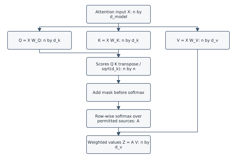
Original course diagram. Follow one destination row: its query scores the source keys, the mask removes forbidden choices, and the normalized weights mix their values. The value path reaches the output without passing through the score calculation. This separation will matter in the Lab.
Lab 06 — Compute and Perturb Attention begins with hand calculation and masking, then implements small arrays using Python’s standard library. Record predictions before checking the answer key. The Lab separates changes to weights in the attention map from changes to the values being mixed.
Several heads write back to the residual stream
A single head produces one distribution over sources for each destination. Every coordinate of that head’s value output uses the same distribution. Several heads allow different projected representations and different distributions to coexist.
For head \(h\), write \(Z^{(h)}=A^{(h)}V^{(h)}\). With \(H\) heads of value width \(d_v\), concatenate their output coordinates and apply a learned output projection:
\[ Y=\operatorname{Concat}(Z^{(1)},\ldots,Z^{(H)})W_O, \qquad W_O\in\mathbb{R}^{Hd_v\times d_{\text{model}}}. \]
Then \(Y\) has shape \(n\times d_{\text{model}}\), appropriate for the residual addition discussed in Lesson 2.1. Concatenation happens along the feature dimension, not along the sequence. Output projection can mix, amplify, suppress, or change the sign of head coordinates. Consequently the final residual update is not constrained to be a convex average of the original residual vectors. PyTorch MultiheadAttention documentation
Imagine a deliberately constructed two-head computation at position 3. One head uses \([1,0,0]\) and carries a feature from position 1; another uses \([0,1,0]\) and carries a different feature from position 2. Concatenation preserves the two outputs separately for \(W_O\) to combine. These are idealized routing patterns for explanation, not measured attention maps. With finite unmasked softmax scores, such exact one-hot patterns are approached rather than attained.
Heads do not arrive with fixed labels such as “grammar” and “facts.” Describing a trained head requires evidence across examples and a specified measurement. Multiple heads can cooperate, overlap, or be unimportant for a particular input.
For our one-head numerical example, choose \(W_O=I_2\). Then \(Y=Z\). If \(X\) is also the residual state in a deliberately simplified block with no normalization, the residual result is \(X+Y\), whose last row is \([5/2,4]\). In a pre-normalized block, add \(Y\) to the original residual state, not automatically to the normalized \(X\).
Contextual computation and stored weights
Consider replacing a token while leaving the checkpoint unchanged. Its residual representation can change; so can its projected key and value. Other positions’ queries can then produce different attention weights and mixtures. Later layers propagate those changes. None of this requires updating a learned parameter.
The reverse distinction matters too. Attention is parameterized by learned matrices, including the projections that determine what is scored and what is written. Calling it “context mixing” should not suggest that attention has no learned structure. Its temporary coefficients \(A_{ij}\) and its stored parameters \(W_Q,W_K,W_V,W_O\) both matter, but on different timescales. The research distinction between query-key and output-value computations is a useful deeper view of these roles. Elhage et al., A Mathematical Framework for Transformer Circuits
At a later layer, source position \(j\) may already contain information gathered from earlier positions. Reading \(v_j\) therefore need not mean reading only token \(t_j\) in isolation. A map records the immediate source position of one mixture; tracing where that source’s contents came from requires looking at preceding computation.
The mask establishes possible routes, not a guarantee that relevant information is recovered. An allowed earlier detail may receive little weight, may be poorly represented in the values, or may be suppressed by downstream transformations. Access and effective use are separate questions.
Self-attention and cross-attention
Self-attention means queries, keys, and values are derived from the same sequence of states. It does not mean each position reads only itself. A causal decoder restricts self-attention to the prefix. An encoder can instead let every non-padding position read the whole input, including positions to its right. BERT is a primary example of a bidirectional Transformer encoder. Devlin et al., BERT
Cross-attention uses queries from one sequence and keys and values from another. The original Transformer’s decoder queries encoder outputs. With \(m\) queries and \(n\) sources, \(S\) and \(A\) have shape \(m\times n\); each row normalizes over its available sources. Vaswani et al., section 3.2.3
Choosing a mask is therefore an architectural and task decision. A translation decoder can read the supplied source sentence while remaining causal over its generated target sequence. “All attention must be triangular” would confuse one important use with the general mechanism.
Positional information also influences practical attention. Our tiny example isolates the arithmetic and includes no separate positional mechanism. Lesson 2.4 will examine positions and modern implementation choices; this lesson’s job is to make the basic computation inspectable.
What an attention map can establish
For a specified input, layer, head, and mask, a faithful plot of \(A\) shows the coefficients used to mix the value vectors. It can reveal an unexpectedly reversed axis, a broken causal mask, or a repeatable pattern worth investigating. Record whether a visualization shows one head or an average across heads; an average can hide distinct patterns.
The map omits the value vectors and output projection. Our example makes that omission concrete. Keep \(Q\), \(K\), and the mask fixed, but replace \(v_2=[0,4]\) with \([0,0]\) after projection. The map remains identical, yet
\[ z_3'=\tfrac14[2,0]+\tfrac14[0,0]+\tfrac12[2,4] =[\tfrac32,2]. \]
Identical maps can accompany different outputs. Conversely, if two sources have identical values, reallocating weight between them while preserving their combined weight leaves this mixture unchanged. Neither statement says that attention weights never matter. Each follows from the full equation \(Z=AV\).
Research on Transformer attention supports examining transformed vectors as well as coefficients: Kobayashi and colleagues showed that vector norms changed conclusions drawn from weight-only analyses of BERT and a translation model. Norms add information but still omit direction, cancellation, and downstream computation. Kobayashi et al., 2020
The broader explanation debate also needs its scope preserved. Jain and Wallace found failures of weight-based explanations in the attention-equipped NLP models they tested. Wiegreffe and Pinter challenged aspects of the tests and argued for explicit definitions and stronger controls. Much of that exchange concerned recurrent models with attention, not a universal evaluation of every modern decoder Transformer. The practical lesson is to test an explanatory claim rather than declare attention always sufficient or always useless. Jain and Wallace, 2019; Wiegreffe and Pinter, 2019
For a causal claim, specify an intervention and an outcome. “Zero this head’s contribution and measure the change in the next-token logit” is testable. “This bright square explains the answer” skips the values, other heads, residual path, MLPs, and later layers. Even a measured ablation effect is conditional on the input, intervention, and metric; it does not automatically establish a unique explanation or broad linguistic role.
Check your understanding
Try these without looking back, then compare your reasoning with the answers.
- \(X\) has shape \(5\times12\), and a head has \(d_k=3\), \(d_v=4\). What are the shapes of \(W_Q\), \(S\), \(A\), and \(Z\)?
- Why does replacing a blocked score with zero fail to implement a causal mask?
- What happens to a source’s normalized weight if its score stays fixed while a competing allowed score increases?
- In the worked example, does \(A_{11}=1\) show that position 1 is more important to the final answer than position 3?
- At position 3, forbid source 2 while preserving all remaining scores and values. Compute the new weights and mixture.
- Can a token change a later position’s output without changing the checkpoint? Can an unchanged attention map establish an unchanged output?
- \(W_Q:12\times3\); \(S,A:5\times5\); \(Z:5\times4\).
- Zero has exponential one. A forbidden source must be excluded from normalization, represented here by negative infinity before softmax.
- It decreases because the denominator increases. Equal allowed scores give a uniform distribution over those sources.
- No. Position 1 has only one allowed source, so its sole coefficient must be one. That says nothing about its downstream importance.
- Remaining exponentials are \([2,0,4]\), giving \([1/3,0,2/3]\) and \([2,8/3]\). Zeroing \(v_2\) instead would preserve \(A\) and give \([3/2,2]\); these are different interventions.
- Yes: activations and mixtures change at inference with fixed parameters. No: values or output projections can change while the map stays the same.
More Learning
- Attention Is All You Need — Vaswani et al. Read section 3.2 beside your hand calculation. Identify the projection, normalization, masking, and multi-head operations before returning to the whole architecture.
- PyTorch scaled-dot-product attention documentation Read the reference pseudocode and mask semantics. Notice the explicit softmax axis and dropout argument; our Lab omits dropout and framework dependencies.
- A Mathematical Framework for Transformer Circuits — Elhage et al. Optional deeper reading on the separate query-key and output-value computations. Pay attention to its simplified model assumptions and different vector convention.
- Attention is Not Only a Weight — Kobayashi et al. Follow the move from plotting scalar coefficients to inspecting the vectors they scale. Ask which information a norm still leaves out.
- Attention is not Explanation — Jain and Wallace Read the experimental setup before generalizing the conclusion. Identify the models, alternative importance measures, and counterfactual tests.
- Attention is not not Explanation — Wiegreffe and Pinter Read alongside the preceding paper. Write one sentence defining the explanatory claim you would actually test and one control it would require.
The next lesson examines the position-wise MLP: what it does with the information represented at each position, and why a coordinate or neuron need not correspond neatly to one concept.