5.2 — Sparse Autoencoders and Learned Features
Module 5 — Mechanistic Interpretability
Search for a more useful coordinate system
In Lesson 2.3, a neuron was a coordinate in a computation, not a guaranteed concept detector. Several properties can share a coordinate, and one property can occupy a direction spread across many coordinates. Lesson 5.1 then gave measurements an address: a checkpoint, computational boundary, token position, and numerical convention. We now ask whether we can learn a useful decomposition of the vectors collected at that address.
A sparse autoencoder, or SAE, is a separate model trained to reconstruct those vectors using relatively few active entries from a larger learned dictionary. The language model can remain frozen throughout. The SAE supplies candidate units for analysis; it does not automatically reveal the unique vocabulary of the language model’s computation.
This distinction makes the method more useful. We can test a decomposition’s reconstruction, sparsity, stability, and relationship to behavior without pretending that a readable label settles every question.
By the end, you should be able to:
- distinguish a basis, an overcomplete dictionary, an SAE latent, and a proposed feature interpretation;
- calculate a sparse reconstruction and its errors;
- explain the roles of the encoder, decoder, regularizer, and decoder normalization;
- compare reconstruction quality with sparsity and held-out feature recovery;
- distinguish a teaching ReLU/L1 SAE from Gemma Scope’s JumpReLU/L0 SAEs;
- interpret a feature display while identifying missing evidence and plausible failures.
Prerequisites are MLPs, Features, and Superposition and Looking Inside a Model. The accompanying Lab 18 trains small synthetic SAEs on a CPU. It does not require downloading Gemma.
Needed now: a linear combination adds scaled vectors; squared reconstruction error adds squared coordinate errors; sparsity counts how many coefficients are active.
Useful refresh: matrix dimensions, optimization with a regularizer, cosine similarity, and train/validation/test separation.
Side trail: conditions for unique sparse recovery, compressed sensing, and gradient estimators for discontinuous functions. We use concrete counterexamples rather than assuming a general recovery theorem.
A dictionary need not be a basis
For an activation \(x\in\mathbb R^d\), collect \(m\) candidate directions as the columns of a matrix \(D\in\mathbb R^{d\times m}\). A reconstruction has the form
\[ \widehat x=b_{\mathrm{dec}}+Dz =b_{\mathrm{dec}}+\sum_{j=1}^{m}z_jd_j. \]
Here \(z_j\) is the coefficient of direction \(d_j\). A basis of a \(d\)-dimensional space has \(d\) independent vectors. A dictionary can have more than \(d\) vectors, making it overcomplete. Its directions then cannot all be linearly independent. This is permitted: we hope that only a small subset is needed for each input.
Sparse coding and dictionary learning long predate language-model interpretability. Sparse coding finds a small set of coefficients for a signal; dictionary learning also learns the directions from data. Classical methods often optimize coefficients separately for each example. An SAE instead learns an encoder that proposes coefficients in a forward pass. Mairal and colleagues, Online Learning for Matrix Factorization and Sparse Coding
Why might this fit language-model activations? The superposition hypothesis proposes that more feature directions can be represented than the space has dimensions when they do not all need to be active together. Toy-model experiments demonstrate conditions under which sparse features are packed this way, with interference and nonlinear filtering. They motivate a search strategy; they do not establish that every model state has one exact sparse semantic decomposition. Elhage and colleagues, Toy Models of Superposition
Nor does “sparse” mean that the observed vector itself contains many zeros. Adding two dense dictionary vectors can produce a dense \(x\) even though only two dictionary coefficients are nonzero.
Work through an exact decomposition
Use this original two-dimensional dictionary:
\[ D= \begin{bmatrix} 1&0&1/\sqrt2\\ 0&1&1/\sqrt2 \end{bmatrix}, \qquad b_{\mathrm{dec}}=0. \]
Each column has unit norm. There are three directions in a two-dimensional space. For
\[ x=\begin{bmatrix}1\\1\end{bmatrix}, \]
both
\[ z_A=\begin{bmatrix}1\\1\\0\end{bmatrix} \quad\text{and}\quad z_B=\begin{bmatrix}0\\0\\\sqrt2\end{bmatrix} \]
reconstruct \(x\) exactly. The first uses two directions; the second uses one. Their numbers of nonzero entries are \(2\) and \(1\), while their sums of absolute coefficients are \(2\) and \(\sqrt2\).
This is already a warning about interpretation. If the data generator produced \(x\) by combining the first two directions, a sparsity objective could prefer the third. A simpler reconstruction is not necessarily a recovery of the original causes.
Now suppose we observe
\[ x'=\begin{bmatrix}1\\0.8\end{bmatrix} \]
and insist on using only the diagonal direction. The best coefficient under squared error is \(z_3=d_3^\mathsf{T}x'=1.8/\sqrt2\), giving \(\widehat x'=[0.9,0.9]^\mathsf{T}\). The squared error is \(0.1^2+(-0.1)^2=0.02\).
Using the first two directions gives zero error but uses two coefficients. Neither result is mysteriously correct. They optimize different combinations of fidelity and economy.
Notice another consequence. Dot products with every decoder direction do not automatically recover valid sparse coefficients. For \(x=[1,1]^\mathsf{T}\), \(D^\mathsf{T}x=[1,1,\sqrt2]^\mathsf{T}\), whose reconstruction is \([2,2]^\mathsf{T}\). Nonorthogonal directions overlap. An encoder must learn how to manage that overlap; it is not simply a list of independent projections.
Complete Part 1 of Inspect Sparse Features. Compare two exact reconstructions, calculate a regularized objective, and predict what information a sparse reconstruction might discard. Record the predictions before training.
The SAE learns a detector and a reconstruction rule
For the teaching model, define
\[ \begin{aligned} z(x)&=\operatorname{ReLU}\left(W_{\mathrm{enc}}(x-b_{\mathrm{dec}}) +b_{\mathrm{enc}}\right),\\ \widehat x(x)&=Dz(x)+b_{\mathrm{dec}}. \end{aligned} \]
The encoder matrix has shape \(m\times d\), the encoder bias has \(m\) entries, and the decoder bias has \(d\) entries. ReLU sets negative preactivations to zero, so the coefficients are nonnegative. Subtracting the decoder bias before encoding is one convention; implementations may instead incorporate that offset into the encoder bias.
An SAE latent consists of an activation function \(z_j(x)\) together with its reconstruction direction \(d_j\). The encoder row determines when it fires. The decoder column determines what vector it contributes. These weights need not be transposes after training.
Early language-model SAE studies fitted sparse reconstructions to internal activations and evaluated whether the resulting units supported more selective descriptions than individual neurons. That is an empirical research program, not a theorem that the training objective produces human concepts. Cunningham and colleagues, Sparse Autoencoders Find Highly Interpretable Features in Language Models
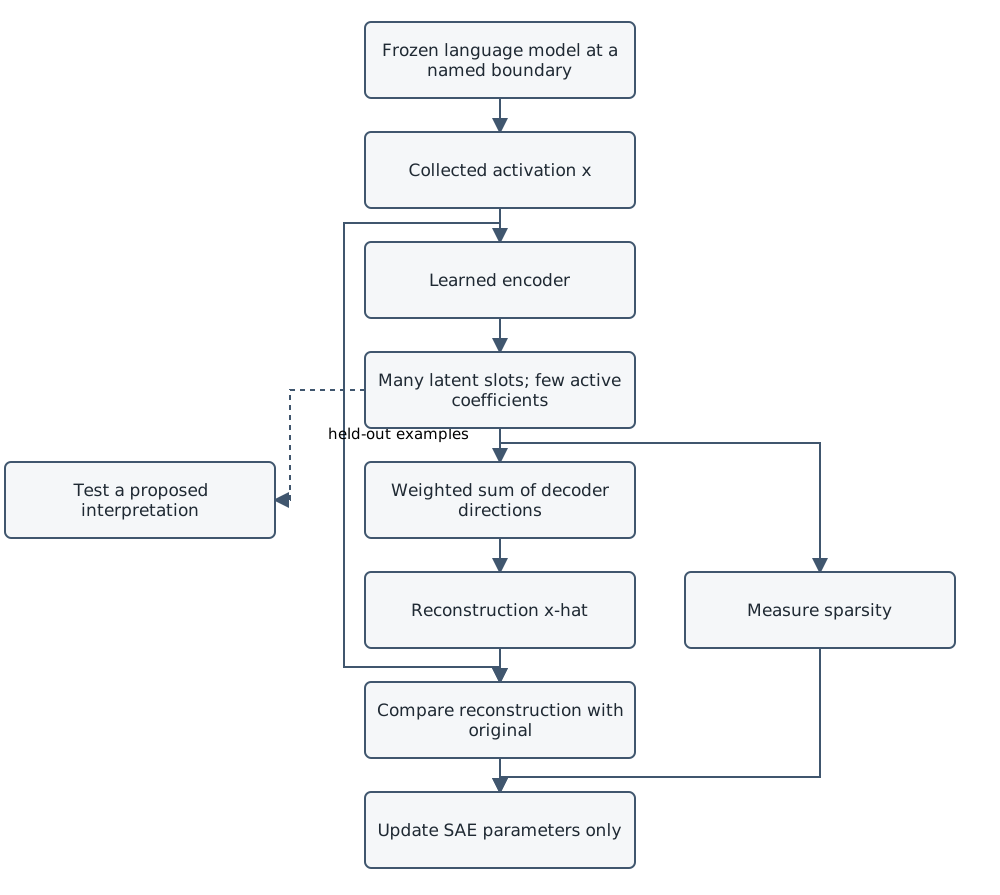
Original course diagram. Training the SAE changes the inspecting model; it does not update the frozen language model.
Prose alternative: Collect vectors from one specified model boundary. Encode each into a larger coefficient vector, reconstruct it as a weighted sum of learned directions, and optimize reconstruction and sparsity. Later, use separate examples to test descriptions of the learned units.
Pay for reconstruction and activity
For a minibatch of \(N\) examples, our teaching objective is
\[ \mathcal L= \frac1N\sum_{i=1}^{N} \left[ \|x_i-\widehat x_i\|_2^2 +\lambda\|z(x_i)\|_1 \right]. \]
The reconstruction term sums over input coordinates before averaging examples. The L1 term sums over latents before averaging examples. Changing either reduction changes the effective strength of \(\lambda\).
The L1 penalty is \(\|z\|_1=\sum_j|z_j|\); here it equals \(\sum_jz_j\). The L0 quantity \(\|z\|_0=\sum_j\mathbf1[z_j\ne0]\) counts active entries. Despite the conventional name, L0 is not a mathematical norm. L1 charges for magnitude, while L0 charges for participation.
For a one-dimensional example with a fixed unit decoder, minimize
\[ (a-z)^2+\lambda z,\qquad z\ge0. \]
Differentiating in the positive region gives \(2(z-a)+\lambda=0\). Including the nonnegativity constraint,
\[ z^\star=\max(0,a-\lambda/2). \]
Thus L1 both removes sufficiently small coefficients and shrinks surviving ones. For \(a=1\) and \(\lambda=0.2\), the optimum is \(0.9\), even though \(z=1\) reconstructs perfectly. This calculation explains one limitation of a convenient sparsity surrogate.
Scaling creates another issue. Replace a decoder direction by \(cd_j\) and its coefficient by \(z_j/c\), with \(c>1\). Their product is unchanged, but the L1 charge decreases. Without controlling decoder scale, optimization can reduce the penalty without learning a meaningfully sparser representation.
Our Lab constrains every decoder column to unit norm, projects its gradient onto the column’s tangent plane, and renormalizes after each update. These are optimization conventions, not proofs of recovery. Decoder normalization, pre-encoder bias, and inactive units are practical concerns in early SAE training work. Bricken and colleagues, Towards Monosemanticity
Training is a separate experiment
With a language model, collect many activations from one consistent boundary and train the SAE on those vectors. Keep the checkpoint frozen. Avoid mixing residual-stream states, MLP hidden values, and normalized branch outputs merely because two arrays happen to share a width.
Separate examples used to fit weights from examples used to evaluate them. If prompts are near duplicates, a row-level random split can exaggerate generalization. Fit any centering or scaling on training data only. Document special-token handling, token positions, precision, and the activation distribution.
In the Lab, the source is simpler: an explicitly planted dictionary generates noisy vectors from sparse nonnegative coefficients. Training receives only vectors, not the planted dictionary or its coefficients. After every SAE has finished, the evaluator can reveal those hidden ingredients and ask whether learned directions resemble them.
This construction gives us a known target for an instructional experiment. It does not recreate language. A successful recovery says something about the selected generator, architecture, optimizer, sample size, and seeds. A failure is also informative: reconstruction may improve while the learned dictionary fails to match the generating one.
Record dead latents as a measurement over a stated sample: for example, no coefficient exceeded the declared activity threshold on 2,048 held-out examples. This is weaker than “never activates anywhere.” A permanently inactive ReLU can receive no ordinary activation-path gradient, while a merely rare latent may be missed by a small sample. Resampling and auxiliary losses are possible training remedies; the Lab intentionally omits them so its small procedure stays inspectable.
Evaluate more than one number
Start with held-out reconstruction error. A useful normalized measure is fraction of variance unexplained:
\[ \mathrm{FVU}= \frac{\sum_i\|x_i-\widehat x_i\|_2^2} {\sum_i\|x_i-\overline x\|_2^2}, \]
where \(\overline x\) is the mean of the evaluation set in this definition. Computing that mean for a metric does not fit the SAE. An FVU below one beats reconstruction by that set’s mean; it need not be positive evidence of meaningful feature recovery. If the denominator is zero, the metric is undefined.
Report activity too: average L0, the distribution of coefficients, and how frequently each latent fires. For floating-point results, state whether “active” means exactly positive or greater than a small threshold. A tiny coefficient might count toward one convention and not the other.
An exact coordinate copy illustrates why reconstruction alone is insufficient. Write each coordinate as
\[ x_k=\operatorname{ReLU}(x_k)-\operatorname{ReLU}(-x_k). \]
A dictionary containing positive and negative coordinate directions can reconstruct any vector exactly with nonnegative coefficients. Nothing in that identity recovers the generator’s preferred directions or a human interpretation.
In our planted experiment, compare learned and generating directions by cosine similarity, report collisions when several generating directions choose the same learned latent, and test whether matched coefficients track held-out generating activity. Do not reward a direction match alone if its encoder fires on unrelated inputs.
For a real language model, another diagnostic replaces \(x\) with \(\widehat x\) and measures changes in model loss or outputs. This tests the consequences of using the reconstruction at that site. It still does not certify every latent’s explanation. SAE evaluation research therefore considers several properties and downstream tests rather than reducing quality to one reconstruction score. Gao and colleagues, Scaling and Evaluating Sparse Autoencoders; Karvonen and colleagues, SAEBench
Complete Parts 2–4 of Inspect Sparse Features. Train the declared small runs, freeze them, and compare held-out reconstruction, activity, and planted-feature matching. Report all runs, including unsuccessful recovery.
A feature description is a hypothesis
Suppose a dashboard’s strongest examples contain web addresses. “URL-related” is a candidate description. It remains unclear whether the unit tracks a protocol prefix, punctuation, a domain suffix, quoted text, or another correlated property.
Top examples are selected precisely because they activate strongly. They help generate hypotheses but cannot establish recall: you have not counted examples of the proposed property on which the latent stays quiet. They can also hide unrelated behavior among weaker activations.
Make an interpretation testable. For the URL example, collect addresses without protocol prefixes, protocol strings outside addresses, ordinary punctuation, quoted and unquoted variants, and unrelated negative examples. Decide which token position matters. Hold back a family of examples while forming the description, then inspect both mistakes and successes on that family.
If a description acts like a classifier, report precision and recall at a declared activation threshold. High precision means activations usually coincide with the proposed property. High recall means most examples of the property activate. Neither follows from a handful of attractive text excerpts.
There are documented failures beyond poor labels. In a Gemma-based first-letter study, a latent that usually tracked words beginning with a particular letter missed some positive cases; other token-aligned latents carried the relevant direction instead. The authors call this feature absorption. A display can therefore look semantically coherent while omitting important cases. Chanin and colleagues, A is for Absorption
Keep “latent” for the learned numerical unit and “interpretation” for your current account of it. A label is neither an architectural name nor a guarantee that the unit has one meaning across distributions. It also does not establish an emotion, subjective experience, intention, or belief inside the model.
More than one decomposition can fit
Some ambiguity is unavoidable. Permuting dictionary columns and applying the same permutation to coefficients changes no reconstruction. Latent 17 in one run therefore need not correspond to latent 17 in another.
Other ambiguity is substantive. If two generating coefficients always equal one another, the data reveal their combined contribution \((d_1+d_2)z_1\). Without additional variation, separating them is underdetermined. More optimization does not supply the missing observations.
Duplicated directions create another exact ambiguity. If \(d_1=d_2\), then \(z_1d_1+z_2d_2=(z_1+z_2)d_1\). Many allocations of nonnegative activity have identical reconstruction and L1 cost. Unit normalization removes a scaling loophole; it does not remove these alternatives.
Increasing dictionary width can change the level of detail, splitting broad patterns among several units. Correlations, noise, regularization, and finite data further influence what gets learned. Compare seeds and settings before treating one dictionary as definitive. Our Lab reports matching collisions rather than silently forcing every planted direction to have a unique winner.
Gemma Scope is a real specimen
The original Gemma Scope release provides pretrained SAEs at multiple sites in Gemma 2: attention-head outputs, MLP outputs, and residual-stream states. Its report includes all layers of the 2B and 9B base models, selected 27B layers, and additional instruction-tuned-model experiments. This lesson uses that named release rather than assuming all later similarly named resources are identical. Gemma Scope report, Sections 2–3
Gemma Scope uses JumpReLU, not our toy’s ReLU:
\[ z_j=a_j\mathbf1[a_j>\theta_j],\qquad a=W_{\mathrm{enc}}x+b_{\mathrm{enc}},\qquad \theta_j>0. \]
Above its learned threshold, a coefficient keeps its preactivation magnitude. The sparsity objective penalizes L0 directly. Because the threshold gate is discontinuous, its training uses straight-through gradient estimators; ordinary differentiation through a hard comparison is insufficient. The JumpReLU work studies this approach as a way to improve the fidelity–sparsity tradeoff and avoid L1’s magnitude shrinkage. Rajamanoharan and colleagues, Jumping Ahead
The released parameters incorporate training-time scaling and the pre-encoder offset for inference. Do not copy our toy preprocessing into that inference path. The report also specifies unit decoder norms during training and projected decoder gradients. Gemma Scope report, Section 3.2 and Appendix A
A useful artifact address includes the model, site, layer, dictionary width, sparsity variant, revision, and latent index. For example, the publisher’s residual-stream model card identifies its demonstration SAE as layer_20/width_16k/average_l0_71 within google/gemma-scope-2b-pt-res. The L0 value is an average activity descriptor, not a promise that every token activates 71 latents. The card also warns of labeling issues and duplicate entries, so record a complete path rather than relying on a friendly name. Publisher model card
Part 5 of the Lab inspects published feature evidence without model downloads. That source-reading exercise and your synthetic training results must remain separately labeled.
Reconstruction is not a causal explanation
An SAE reconstruction can be written \(x=\widehat x+e\), where \(e\) is its residual error. Replacing \(x\) by \(\widehat x\) removes every part of that error, not just one proposed concept. A subsequent behavior change therefore mixes the effects of many omissions.
Removing one latent while preserving the original error instead gives \(x'=x-z_jd_j\). This specifies an intervention more narrowly, but it can still disturb correlated information or create an unusual state. Its effect belongs to that exact edit, input distribution, site, and output measure.
Lesson 5.3 develops these tests. For now, keep the evidence categories from Lesson 5.1: a sparse decomposition, an interpretation supported by examples, and a controlled causal account are different achievements. An SAE provides useful candidates for the next experiment, not a shortcut around it.
Check your understanding
Try these without looking back.
- How can a 16-dimensional vector have a dictionary of 64 directions?
- Why is \(D^\mathsf{T}x\) not generally a valid sparse decoding?
- What loophole does decoder normalization close under an L1 objective?
- Why can L1 hurt reconstruction even for a coefficient that remains active?
- What does a dead-latent count actually measure?
- Why can excellent FVU coexist with poor planted-feature recovery?
- What evidence is missing from a page of top-activating examples?
- Which two central choices distinguish our toy from Gemma Scope?
- Why does setting one latent to zero not automatically erase one concept?
- A dictionary may be overcomplete and dependent; each input uses a subset.
- Nonorthogonal directions overlap, so independently projected contributions can double-count.
- Enlarging decoder columns while shrinking coefficients preserves reconstruction but reduces L1.
- L1 charges magnitude as well as encouraging zeros.
- Inactivity under a stated threshold on a stated evaluation sample.
- Many decompositions, including coordinate copies, reconstruct well without recovering generating directions.
- Recall, counterexamples, performance outside the selected examples, and causal evidence.
- ReLU versus JumpReLU; L1 magnitude penalty versus L0 activity penalty.
- The latent can mix properties, a property can occupy several latents, and the edit can affect downstream computation in other ways.
More Learning
- Towards Monosemanticity. Read the problem setup and one feature case study. Separate the numerical unit from the evidence for its label.
- Gemma Scope. Read Sections 2 and 4, then locate one exact training site in Section 3.
- Jumping Ahead. Follow the threshold rule and ask why its gradient needs special treatment.
- A is for Absorption. Follow the first-letter example as a counterexample to complete concept detectors.
- SAEBench. Compare evaluation questions rather than searching for one winning scalar.
- Online Learning for Matrix Factorization and Sparse Coding. Optional mathematical background on dictionary learning before language-model applications.