5.1 — Looking Inside a Model
Module 5 — Mechanistic Interpretability
Turn an internal picture into a testable claim
An activation heatmap can be striking while answering a surprisingly narrow question: which numbers occurred at one place in one computation? To explain a model, we must connect those numbers to defined inputs, outputs, and possible mechanisms. This lesson builds that connection carefully.
Lessons 2.1–2.3 introduced the residual stream, attention, and MLPs. Module 4 separated the model from the surrounding product and agent harness. Here we inspect a model’s forward pass. We are not inspecting a product’s hidden system message, retrieving training documents, or reading a literal transcript of thoughts.
The practical sequence is to locate a boundary, observe it without changing the computation, validate the measurement, and ask a question that the evidence can actually answer. A small model is sufficient to learn this discipline. Interesting-looking output is optional; a reliable measurement is essential.
By the end, you should be able to:
- give an activation an exact address in a forward pass;
- distinguish observation hooks, stored activations, and generation caches;
- compare vectors with norms, cosine similarity, and projections;
- implement and qualify a logit-lens readout;
- explain what held-out probe performance does and does not establish;
- distinguish a descriptive observation from evidence of causal use.
Needed now: vector norms, dot products, projections, and cosine similarity. We derive a complete numerical example below.
Useful refresh: affine maps, softmax, train/test separation, and regularized regression.
Side trail: causal mediation, statistical power, and high-dimensional geometry. These deepen the analysis but are unnecessary for the core Lab.
Give every tensor an address
“Layer 3 activation” is incomplete. Does it mean the third block’s input, its MLP hidden values, its attention output, or the stream after residual addition? Does “3” use zero-based indexing? Has normalization already happened?
For each observation, record the checkpoint and revision, implementation version, exact token sequence, batch index, token position, block index, module path, and boundary. Also record the tensor’s shape and numerical type. A useful description is: “For prompt P2, batch 0, final input position 11, zero-indexed block 2, raw post-block residual vector, before any final normalization.” The position number here illustrates the record format; an actual experiment must obtain it from tokenization.
With batch size \(b\), input length \(n\), and residual width \(d\), a residual activation has shape \((b,n,d)\). Selecting one prompt and one position gives a \(d\)-dimensional vector. A block’s MLP hidden activation can instead have width \(m\). An attention matrix has source and destination axes as well as batch and head axes. Similar names do not make these arrays interchangeable.
Position is especially important in a causal decoder. The logits at input position \(i\) score the token after that position, using its permitted prefix. They are not probabilities assigned to the token currently occupying row \(i\). For next-token inspection, selecting the final nonpadding position is convenient. If two prompts have different lengths, their final positions need not have the same numerical index.
Repeated token IDs also need separate addresses. Two occurrences of a colon share an input embedding, but their later representations can depend on different prefixes. Conversely, matching a final token ID controls that embedding without controlling the entire context, token count, or position.
Hooks observe a running computation
A hook is a callback attached to a computational boundary. A forward pre-hook observes a module’s inputs before that module runs; a forward hook observes its returned output. Some hook interfaces also permit replacing values. For observation, leave the computation untouched and return None. An accidental replacement turns the experiment into an intervention. PyTorch supplies removable hook handles; use them to guarantee cleanup. PyTorch module hooks
A module name alone does not specify how to extract its result. Some modules return a tensor, others a tuple or structured object. Inspect the pinned implementation and assert the expected type and shape. A generic “take element zero” recipe can either select a tuple’s tensor or accidentally discard a tensor’s batch dimension.
An activation cache in this lesson is a record you make of selected measurements. It may be a small dictionary of copied vectors, with descriptive keys and associated metadata. It is different from the key–value cache used to avoid repeating attention work during generation. We disable generation caching in the Lab because we want simple full-prefix passes, not because all caches are inherently unreliable.
Detach recorded values from any gradient graph and clone the required slice so later operations cannot change the saved record through shared storage. Do not keep an entire sequence tensor alive merely to retain one row. Clear per-prompt records before each run. If a module is called unexpectedly twice, stop and investigate rather than silently overwriting its first observation.
A successful instrumented pass is not enough. Compare it with an uninstrumented baseline on exactly the same input. Then remove the hooks and repeat the baseline. These checks test whether the observer changed the result or left state behind.
Locate the boundaries in a real block
The Lab reuses Pythia-14M at revision 94f7c35d5e9f2e9bac8ca839329f505b4d007d5d: six blocks, residual width 128, MLP width 512, and parallel residuals. Its input and output embedding weights are not tied. These are checkpoint-specific facts, not a template for every Transformer. Pinned publisher configuration
Write \(R_\ell\) for the raw sequence-shaped input to block \(\ell\). In this architecture,
\[ R_{\ell+1}=R_\ell+ A_\ell(N_{\ell,A}(R_\ell))+ M_\ell(N_{\ell,M}(R_\ell)). \]
The branches read separately normalized versions of the same raw input. The MLP does not read its own block’s attention-updated state. At the end, final normalization \(N_f\) precedes the vocabulary head. The versioned GPT-NeoX implementation establishes these boundaries. Transformers v4.57.1 source
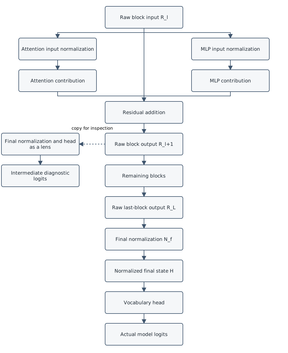
Original course diagram for the Lab specimen. The dotted route records an auxiliary readout; it does not replace the model’s remaining blocks.
Prose alternative: Preserve the raw input for a skip path. Normalize it separately for attention and the MLP, then add both contributions to the raw input. After all blocks, normalize once and project into vocabulary space. An intermediate lens applies that final readout to a copied earlier state while leaving the full forward pass intact.
Three common measurements now have distinct meanings. A residual vector is the accumulated state at a specified boundary. An attention contribution is what its branch writes back after mixing and projection. An MLP hidden vector is the expanded representation inside that branch, before its output map returns to residual width. Their norms cannot be compared as if they were three measurements of the same object.
Attention weights alone omit the values being mixed and the output projection. Large attention to a position therefore does not, by itself, explain the final answer. Likewise, a large MLP activation omits its output direction and downstream use. These are useful observations, provided the question matches the measurement.
Refresh the geometry with an exact example
For vectors \(x,y\in\mathbb R^d\), the dot product and Euclidean norm are
\[ x^\mathsf{T}y=\sum_jx_jy_j, \qquad \|x\|_2=\sqrt{\sum_jx_j^2}. \]
For nonzero vectors, cosine similarity divides alignment by both lengths:
\[ \cos(x,y)=\frac{x^\mathsf{T}y}{\|x\|_2\|y\|_2}. \]
It is undefined when either norm is zero. Replacing that case with a reported similarity of zero invents a measurement. Software may stabilize denominators internally; your report should still identify zero-vector cases explicitly.
For a nonzero direction \(q\), the vector projection onto its span is
\[ \operatorname{proj}_q(x)= \frac{x^\mathsf{T}q}{q^\mathsf{T}q}q. \]
This differs from the signed scalar coordinate \(x^\mathsf{T}\hat q\), where \(\hat q=q/\|q\|_2\). One is a vector; the other is a number.
Consider this original arithmetic example:
\[ x=\begin{bmatrix}2\\1\\2\end{bmatrix},\quad y=\begin{bmatrix}1\\2\\2\end{bmatrix},\quad q=\begin{bmatrix}1\\-1\\0\end{bmatrix}. \]
Both state norms are \(3\), their dot product is \(8\), and their cosine is \(8/9\). Yet their coordinates along \(\hat q\) are \(1/\sqrt2\) and \(-1/\sqrt2\). Their projections are
\[ \operatorname{proj}_q(x)= \begin{bmatrix}1/2\\-1/2\\0\end{bmatrix},\qquad \operatorname{proj}_q(y)= \begin{bmatrix}-1/2\\1/2\\0\end{bmatrix}. \]
Much of each vector is shared, while this particular direction reverses sign. A high cosine does not imply agreement on every downstream question.
Give a hand-constructed three-token vocabulary the output map
\[ U=\begin{bmatrix}2&0&0\\0&2&0\\0&0&1\end{bmatrix}, \qquad z=Ur, \]
with rows corresponding to tokens A, B, and C. There is no normalization or bias in this toy. Then
\[ z(x)=[4,2,2]^\mathsf{T},\qquad z(y)=[2,4,2]^\mathsf{T}. \]
The top token switches from A to B. Softmax gives the top token probability \(e^2/(e^2+2)\approx0.787\) in either case. The A-versus-B logit difference is \(2q^\mathsf{T}r\), which changes from \(2\) to \(-2\). We can explain that change exactly because the complete readout is specified.
Notice also that \(\|y-x\|_2=\sqrt2\). Distance, cosine, projection, and output score each answer different questions. None supplies a semantic interpretation of \(q\). Calling it a “confidence direction” would add a claim that this arithmetic never tested.
Read intermediate states with a logit lens
The logit lens uses the model’s output readout to turn intermediate residual states into vocabulary scores. The original named presentation by nostalgebraist used GPT-2 and illustrated how these readouts changed across depth. It is a useful diagnostic idea, not evidence that every model maintains a readable sentence at every layer. Interpreting GPT: the logit lens
Keep our column-vector convention. Let \(r_\ell\) be one selected raw residual vector, and let \(U\) have shape \(V\times d\). For the Lab’s bias-free vocabulary head, define
\[ \widetilde z_\ell=U N_f(r_\ell). \]
At the final raw state \(r_L\), this matches the model’s actual output computation. Earlier in the stack, it is a diagnostic that skips remaining blocks. It asks what the final readout produces from this earlier vector, rather than what the full model will necessarily output.
Use the checkpoint’s actual final normalization and output head, including their learned parameters. Do not substitute unit-length normalization for LayerNorm, use the input embedding table because its shape looks convenient, or silently omit an output bias in an architecture that has one. Shape compatibility is weaker than computational equivalence.
There is a particularly easy boundary error. Suppose the capture already contains \(h=N_f(r_L)\). Then the correct reconstruction is \(Uh\), not \(UN_f(h)\). Reapplying normalization is generally a different function because learned scales, offsets, and numerical stabilizers are part of it. Label raw and normalized records separately instead of trying to infer their meaning from their magnitudes.
A second trap concerns addition. In general,
\[ N_f(r+a+m)\ne N_f(r)+N_f(a)+N_f(m). \]
Applying the lens separately to branch contributions and summing the results therefore does not reconstruct the lens of their sum. A contribution’s readout also is not its causal effect after subsequent blocks recompute. Derivations that hold a normalization scale fixed need to disclose that assumption.
Why should an early lens work at all? Residual connections provide shared-width states, and some trained representations are usefully readable with the final map. But the head was trained on final-space representations; earlier states can have different scales, offsets, or feature arrangements. Poor early candidates need not mean the relevant information is absent. Good candidates need not mean the later computation uses precisely that readout.
The tuned lens addresses this mismatch by fitting an affine translator at each layer before the final readout, with the base model frozen. Belrose and colleagues train translators to approximate the model’s final output distribution and separately investigate causal fidelity. This improves a readout in their experiments; training another decoder is not an automatic proof of the base model’s mechanism. Tuned Lens, Sections 2–4
Our Lab uses an untrained logit lens. It reports top candidates rather than claiming to reconstruct hidden reasoning. Keep token IDs alongside decoded pieces: whitespace, special tokens, and byte fragments can make attractive word-only displays misleading. A probability computed over five retained candidates is also not the full-vocabulary probability. Compute the proper denominator or report logits instead.
Complete the core of Inspect Activations. Validate the boundaries and final-logit reconstruction before interpreting any layer-by-layer candidates. No particular model answer or pleasing progression is required.
A probe learns a readout
A probe is a separate predictor trained on activations to predict a label. A linear binary probe might use \(w^\mathsf{T}r+b\), with a threshold or logistic transformation. The frozen base model supplies \(r\); fitting \(w,b\) trains the probe rather than updating the base model.
Suppose the label says which of two boxes a prompt describes as red. Successful prediction on unseen examples would show that the chosen representation supports that readout under the tested distribution. It would not establish a unique “red box neuron,” nor that the language model uses this particular readout to produce its next token.
Probe design can manufacture apparently impressive results. If red and blue examples use different final tokens, the input embedding may reveal the label without any contextual computation. If near-identical templates occur in training and testing, a probe may exploit their surface patterns. If you inspect many layers and report only the best held-out score, the held-out set has become part of model selection.
Before extracting activations, fix the label, examples, split, boundary, probe capacity, regularization, and metric. Split by template or family when the claim concerns transfer beyond those templates. Fit centering, scaling, and other preprocessing on training data only. Keep the held-out labels out of fitting and selection.
Include an input-embedding or token-identity baseline, class-balance baseline, and shuffled-training-label control. These answer different questions. A shuffle can reveal instability or capacity to fit arbitrary assignments; it does not rule out every systematic confound. Hewitt and Liang’s control-task study makes the broader point that probe accuracy needs context about what the probe itself can learn. Designing and Interpreting Probes with Control Tasks
A tiny dataset is appropriate for learning the method, but not for a broad representation claim. Report counts, errors, and individual failures. A weak result can mean poor representation, an unsuitable boundary, insufficient data, or an inadequate readout. It does not establish that the model lacks the property altogether.
Separate readout from use
Consider a direction whose projection correlates with a correct answer. Three explanations remain possible: the model uses that direction; another correlated variable drives the answer; or both reflect a shared earlier computation. Observation alone cannot decide among them.
An intervention changes an internal quantity and recomputes downstream behavior. If removing a direction changes an output metric, that is evidence about the effect of that specified manipulation. It still requires controls: perhaps the edit damages unrelated information, produces an unusual state, or changes scale rather than the hypothesized variable. Conversely, a null result may reflect redundancy or an ineffective manipulation. Lesson 5.3 develops these questions.
Keep five evidence categories separate:
- Observed quantity: a named vector, norm, attention coefficient, or candidate score occurred on a recorded input.
- Derived readout: a stated calculation, such as a projection or lens, transforms that observation.
- Predictive association: a fixed readout predicts a label on a declared held-out distribution.
- Controlled intervention: changing a specified quantity changes a declared downstream measure relative to controls.
- Mechanistic account: a proposed computation explains several observations and predicts additional tests, including relevant interventions.
These categories describe claims, not a score awarded to a visualization. An exact reconstruction can establish that your instrumentation matches the implementation without explaining a linguistic behavior. A causal effect can be real without making the component a uniquely necessary explanation.
A good report therefore says “the paired cosine decreased at this boundary,” then offers competing explanations and a next test. It does not jump directly to “the model understood the contrast here.”
Keep the instrument honest
Evaluation mode and gradient disabling solve different problems. Use both: evaluation mode changes modules such as dropout, while inference mode avoids gradient bookkeeping. Neither turns floating-point execution into a universal guarantee of bitwise reproducibility. Record the runtime, device, dtype, attention backend, thread settings, and seeds. PyTorch inference mode; reproducibility guidance
Hooks, tensor copies, and requesting attention matrices can change memory use or execution paths. Do not treat instrumented timings as ordinary inference timings. Keep the baseline and observed pass on the same backend; compare numerical outputs with a tolerance declared before the run and report maximum errors. Cleanup belongs in a guaranteed path even when an assertion fails.
Finally, preserve the experiment’s limits. Save the prompts and positions you actually used, failed checks, and whether each result is analytical or measured. The goal of looking inside is to make a claim more accountable. More captured numbers are useful only when they improve that accountability.
Check your understanding
- Why is “the output of layer 4” an insufficient capture description?
- Calculate \(\operatorname{proj}_q(y)\) and the A-versus-B logit difference in the worked example.
- Can two vectors have equal norms and high cosine while giving different top tokens?
- You capture the final LayerNorm’s output. Which operation reconstructs logits?
- Why can normalized branch readouts fail to add up to the block readout?
- A probe performs well on random example splits but poorly on held-out templates. Which claim has weakened?
- Does a failed early logit lens show that the state contains no useful answer information?
- Does an output-changing ablation alone identify a unique semantic mechanism?
- Specify the checkpoint, implementation, token sequence and position, indexing convention, module, return value, and location relative to normalization and addition.
- The projection is \([-1/2,1/2,0]^\mathsf{T}\); the difference is \(2q^\mathsf{T}y=-2\).
- Yes. Our vectors both have norm \(3\), cosine \(8/9\), and different top tokens under the stated readout.
- Apply the actual vocabulary head directly. Do not apply final normalization again.
- Normalization is not additive; its statistics depend on the complete input. The same caveat applies before making a causal interpretation.
- Transfer beyond familiar templates. Random-split accuracy may reflect template-specific cues; it has not demonstrated the intended generalization.
- No. The final readout may be unsuitable for that intermediate representation.
- No. It establishes an effect of the specified manipulation under the tested conditions; specificity, collateral damage, redundancy, and alternative mechanisms still need examination.
More Learning
- GPT-NeoX implementation, Transformers v4.57.1. Trace the block, final normalization, and vocabulary projection against the original diagram above.
- PyTorch module hooks. Read the return-value and removal rules before instrumenting a model.
- nostalgebraist, Interpreting GPT: the logit lens. The original named presentation. Treat its GPT-2 observations as a particular study rather than expected outputs for this Lab.
- Belrose and colleagues, Eliciting Latent Predictions from Transformers with the Tuned Lens. Compare an untrained readout, a trained translator, and the paper’s additional causal tests.
- Hewitt and Liang, Designing and Interpreting Probes with Control Tasks. Explain why accuracy alone can conceal what the probe learned.
- PyTorch reproducibility guidance. Separate same-environment repeatability from portability across versions and devices.