5.3 — Steering, Ablation, and Causal Intervention
Module 5 — Mechanistic Interpretability
A change is evidence, but evidence of what?
Suppose an internal vector is larger on favorable reviews than unfavorable ones. That is an observation. Suppose a probe predicts the review category from that vector on unseen examples. That establishes useful predictive information under the probe’s evaluation. Now suppose we add a chosen direction to the model’s running computation and its next-token scores change. We have performed an intervention.
The last result is stronger in one respect: we controlled a cause of the changed computation. It is still narrower than “we found the model’s sentiment mechanism.” The edit may exploit an output-sensitive direction, disrupt several representations simultaneously, or work only with a particular sentence ending. Reliable interpretation depends on specifying the change, comparison, and claim together.
Lesson 5.1 taught observation boundaries; Lesson 5.2 introduced learned feature dictionaries. Here we move from looking to manipulating. We will build a direction from contrasting activations, add or remove components, examine forced routing, and design controls. Lab 19 implements a small intervention in the same bounded Pythia checkpoint used earlier. It does not promise a striking behavioral result.
By the end, you should be able to construct and normalize a contrastive direction, distinguish subtraction from projection removal, give an intervention an exact computational address, measure a paired output effect, and state a defensible causal conclusion.
Needed now: vector subtraction, averaging, Euclidean normalization, projection, and differences in measured outcomes. We work through each as it becomes useful.
Useful refresh: dot products, logits and softmax, nonlinear functions, and discovery/test separation.
Side trail: causal mediation and statistical inference. The central discipline comes first: define what changed and what comparison supports your conclusion.
Construct a direction from a contrast
Let \(r_k^+\) and \(r_k^-\) be activations collected from the positive and negative members of pair \(k\). Both must belong to the same checkpoint, layer, boundary, and position-selection rule. Positive means the category we name positive; it is not a value judgment or proof that the model possesses a positive state.
Subtract corresponding coordinates:
\[ d_k=r_k^+-r_k^-. \]
If the first coordinate rises by two and the second falls by one, the difference contains \([2,-1]\), regardless of the original vectors’ lengths. Subtraction describes a displacement in this representation space. Reversing the pair reverses its sign.
Average several paired differences:
\[ d=\frac1K\sum_{k=1}^K d_k =\left(\frac1K\sum_k r_k^+\right) -\left(\frac1K\sum_k r_k^-\right). \]
With equally weighted complete pairs, this is the difference between category means. Pairing still matters scientifically: corresponding examples can share a topic, format, or question. The equality does not make a badly confounded dataset well controlled.
Imagine favorable contexts always discuss restaurants while unfavorable contexts always discuss software. Their mean difference could contain topic, vocabulary, punctuation, and evaluative information together. Averaging reduces some idiosyncratic variation; it does not automatically subtract a confound that consistently accompanies the label. Design varied, meaningfully paired examples before naming the resulting direction.
Activation Addition established a practical approach using activation contrasts to influence subsequent model output. Contrastive Activation Addition, or CAA, aggregates paired differences. Panickssery and colleagues studied Llama 2 Chat using answer-conditioned contrast sets, multiple-choice evaluation, and open-ended responses. Those are findings about their specified models and procedures. Our tiny prefix-based Lab is an instructional adaptation, not a reproduction of their reported performance. ActAdd, v5; CAA, v4
Separate a direction from its scale
A raw mean difference carries both orientation and length. To isolate orientation, calculate
\[ \|d\|_2=\sqrt{\sum_j d_j^2},\qquad u=\frac{d}{\|d\|_2}. \]
Then \(\|u\|_2=1\), and an addition \(\alpha u\) has norm \(|\alpha|\). A zero vector has no defined orientation. A nearly zero vector can amplify rounding or measurement noise when normalized; stop and inspect it rather than calling numerical residue a discovery.
Normalization changes the meaning of the coefficient. In \(r'=r+\beta d\), doubling the discovery contrast norm doubles the applied perturbation at fixed \(\beta\). In \(r'=r+\alpha u\), the coefficient directly specifies perturbation length. Neither convention is inherently correct. Record which one you use so another experimenter can reproduce the dose.
For an exact example, let two contrast vectors be \([2,0]^\mathsf{T}\) and \([0,2]^\mathsf{T}\). Their mean is \(d=[1,1]^\mathsf{T}\), so \(u=[1,1]^\mathsf{T}/\sqrt2\). Adding \(\sqrt2u\) adds one to each coordinate. These numbers are a constructed geometry exercise, not observed model activations.
An absolute perturbation of length one may be tiny at one boundary and large at another. It is useful to report \(\|\Delta r\|_2/\|r\|_2\) alongside the absolute norm. This is a size description, not a guarantee that the edited state remains natural or harmless. An important readout can be sensitive to a small, precisely aligned displacement.
Complete Lab 19, Part 1. Compare adding a fixed vector, subtracting it, and removing a projection. Explain the difference before using a hook to change a real model.
Every intervention needs a computational address
“Add the vector at layer three” is not reproducible. Specify the block index convention, module, input or output boundary, token positions, batch rows, normalization status, and how often the operation occurs. Also identify the checkpoint, implementation, numerical precision, and coefficient.
For our six-block Pythia specimen, block 2 means the third block. We edit its raw output after residual addition, at the final input token only. The remaining three blocks and the final normalization then process the changed state. The checkpoint uses parallel residuals, with attention and MLP contributions computed from separately normalized versions of the same block input. Pinned checkpoint; implementation v4.57.1
Editing the block input would also change both branches’ calculations inside that block. Editing only the MLP output changes one contribution. Editing the raw block output changes their accumulated result. Editing after final normalization bypasses all remaining Transformer blocks. These locations can have the same width while testing different computational hypotheses.
Position matters equally. Changing the final prefix position once measures its effect on the next-token distribution in this setup. Reapplying an edit during generation changes a sequence of computations. Editing every position can also change what later attention reads from earlier positions. Such procedures are related experiments, not interchangeable implementations.
A direction extracted at one site is not automatically portable to another. Dimensions can match while meanings, typical scales, and downstream transformations differ. Treat cross-layer or cross-model transfer as a separate tested claim.
Addition, subtraction, and ablation ask different questions
Activation addition replaces \(r\) with \(r+\alpha u\). Using a negative coefficient moves in the opposite geometric direction. It does not guarantee the opposite behavioral effect: the rest of the model is nonlinear, and the two edited states can enter different computational regimes.
Directional ablation removes the component along a unit vector:
\[ c=u^\mathsf{T}r,\qquad r_{\perp}=r-cu. \]
Here \(c\) is a signed scalar, the coordinate of \(r\) along \(u\). The replacement satisfies \(u^\mathsf{T}r_{\perp}=0\) in exact arithmetic. Unlike subtracting \(\alpha u\), it uses a coefficient determined by the current state. If \(c\) is negative, removing the component requires adding a positive multiple of \(u\).
A centered alternative removes \(u^\mathsf{T}(r-\mu)\) rather than \(u^\mathsf{T}r\), retaining the reference mean’s coordinate. These are different interventions. The reference mean must come from a declared dataset; choosing it after seeing results adds another researcher decision.
Unit ablation might set one MLP hidden activation to zero. Branch ablation might replace an entire attention or MLP contribution with zero. Neither is equivalent to zeroing the residual stream: the latter also erases accumulated information carried by the skip path. “Ablated the layer” conceals too much to be a useful methods description.
Replacement need not mean zero. Mean ablation inserts a reference average; resampling inserts a value from another example. A value normal in its original context can still be an unnatural combination with the receiving prompt’s other activations. Always state the replacement distribution and how it was chosen.
SAE features add another distinction. Removing a decoder direction from the residual stream is not generally the same operation as setting its encoder coefficient to zero and decoding again. Nonorthogonal dictionary directions can overlap, and reconstruction has an error term. Preserve the difference between intervening on the original computation and intervening on a reconstruction.
An exact effect does not require a semantic story
Take the original toy
\[ x=[2,1]^\mathsf{T},\quad u=[1,0]^\mathsf{T}, \quad s(x)=x_1+2x_2. \]
The baseline score is four. Adding \(u\) changes it to five; subtracting \(u\) changes it to three. Removing its projection gives \([0,1]^\mathsf{T}\) and score two. Projection removal has twice the perturbation norm of either fixed addition, even though all three use the same direction. The positive and negative fixed additions have equal norms.
For a linear readout \(s=w^\mathsf{T}x\), addition has the exact effect
\[ s(x+\alpha u)-s(x)=\alpha w^\mathsf{T}u. \]
Magnitude and alignment both matter. A large displacement orthogonal to \(w\) has no immediate effect on this score. A small aligned displacement can matter more. This recovers the lesson from MLP read/write vectors: activation size alone does not rank causal importance.
For a nonlinear downstream function \(F\), we must evaluate \(F(x+\alpha u)\) rather than subtract an old contribution from the final output. Downstream attention, normalization, and nonlinearities can all respond to the changed state. The toy’s closed-form answer teaches bookkeeping, not a shortcut for predicting a trained Transformer’s intervention result.
Forced routing changes which computation runs
A mixture-of-experts layer introduces another intervention target. In a simplified sparse layer,
\[ y=\sum_{e\in S(x)}g_e(x)E_e(x), \]
where the router chooses a set \(S(x)\), expert functions produce vectors, and gate values weight those outputs. Sparse routing architectures make selection, weighting, and capacity handling part of the computation. Switch Transformers
Forcing expert 3 can mean several things: replacing the selected index while keeping the old gate weight, setting the new gate to one, changing router logits and rerunning selection, or substituting the expert output afterward. These interventions need not agree. With multiple selected experts, renormalization can change all their contributions. Capacity limits and dropped tokens add further distinctions.
Ask a precise question, such as whether replacing one selected expert’s contribution with another’s changes a predefined score. Record routing decisions, weights, capacity behavior, and output. Compare with an unchanged-route control. Do not infer that a heavily selected expert is necessary for a topic without such tests, or that forcing another route preserves the model’s normal operating conditions.
Pythia-14M is dense. Lab 19 therefore does not pretend to run a routing intervention. The routing trace in Module 2 supplies a place to apply this reasoning without downloading a new expert model.
Keep discovery separate from the causal test
A good experiment has several stages, and each answers a different question.
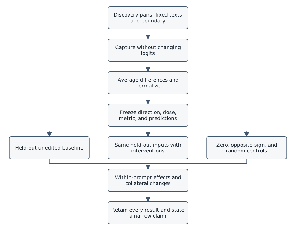
Original course diagram. The freeze separates constructing a candidate from evaluating it. Prose alternative: capture discovery activations, derive a vector, record a complete plan, and only then compare held-out baselines, interventions, and controls. Report their differences together.
The discovery set may legitimately guide a choice of direction, layer, or dose. Every choice must be disclosed. Once held-out results guide another choice, those examples have become development data. Renaming them “test” does not restore independence.
Our Lab avoids a large search: one preselected block, three discovery pairs, two fixed addition sizes, and one random direction. It preserves positive-context-minus-negative-context orientation even if the pilot behaves inconveniently. This small design is pedagogical rather than statistically powerful, but its decision trail is inspectable.
Complete Lab 19 through Part 5. Confirm that capture does not change logits, test cleanup after an intentional exception, derive the direction from discovery alone, and write signed predictions before inspecting held-out model outputs.
Measure an effect without changing the question
Choose an outcome before the test. For candidate next tokens \(a\) and \(b\), use a logit difference
\[ y(x)=z_a(x)-z_b(x),\qquad \Delta y(x)=y_{\mathrm{intervened}}(x)-y_{\mathrm{baseline}}(x). \]
This is a paired comparison: the prompt, weights, and decoding position are held fixed while the intervention changes. Average the differences over declared prompts, but keep individual values. An average of zero can conceal large opposing effects.
Softmax gives \(p(a)/p(b)=\exp(z_a-z_b)\), so this logit difference is the log probability ratio for those two tokens. It is not the absolute probability of either token, and it ignores other possible answers. Both tokens can remain extremely unlikely while their ratio changes substantially.
Verify tokenization. “Good” and “ good” need not identify the same token. A phrase split into several tokens requires a sequence-scoring procedure, not casually selecting the first piece. The Lab avoids that added experiment by requiring two verified single-token candidates.
A logit movement is an output-distribution effect; it need not change the greedy token. Conversely, a tiny movement near a tie can change the greedy answer. Generated-text quality, task accuracy, and judge ratings ask further questions and introduce additional choices. Do not swap metrics after seeing which creates the strongest story.
Zhang and Nanda found that activation-patching conclusions can depend on metric and corruption choices. That result motivates reporting how a score is defined rather than treating an intervention heatmap as method-independent evidence. Activation-patching best practices, v2
Controls test rival explanations
A no-hook baseline establishes the original output. An observation-only pass tests whether measurement itself changes it. A zero-addition hook exercises replacement machinery while requesting no numerical intervention. An unhooked repeat afterward checks restoration. If these fail, troubleshoot the apparatus before discussing semantic mechanisms.
An opposite-sign control asks whether the effect depends on direction, rather than merely perturbing the computation. Symmetry is informative but not guaranteed. A fixed random direction, normalized to the same perturbation length, asks whether an arbitrary equal-sized edit has a comparable effect. One random direction does not describe the distribution of random effects.
Dose controls reveal another ambiguity. If doubling the change strengthens the target score but damages unrelated predictions, the intervention has traded one measured property against others. If projection ablation uses a much larger displacement than addition, its larger effect cannot fairly be credited entirely to a better-targeted operation.
Prompt controls challenge surface explanations. Shared suffixes constrain token identity at the measured position. Varied topics reduce one kind of confounding. New phrasings, swapped labels, and examples that separate evaluative meaning from particular words offer further tests. None should be silently added to the confirmatory set after an appealing observation.
Finally, preserve failure cases. Excluding prompts because the baseline is weak, the sign reverses, or the intervention produces strange output changes the evidence. You may analyze a clearly labeled subgroup, but the original complete result must remain visible.
Distribution shift exists inside the network too
Language-model activations occupy a structured subset of possible vectors under ordinary inputs. An edited state may be mathematically valid while being unlike the combinations the network encountered in training. Calling this “off-manifold” is a useful warning, not a claim that we know the exact manifold or can calculate distance to it from a norm alone.
Normalization can change relative coordinates after an edit. Later nonlinearities can amplify, suppress, or redirect it. A surprising failure might reflect damage from an unnatural state rather than removal of a uniquely meaningful representation. Successful steering can also exploit an unusual state rather than reproduce a naturally occurring mechanism.
Inspect collateral effects: distributional change over the full vocabulary, off-task examples, and dose sensitivity. A KL divergence from baseline summarizes one kind of output change, but large KL does not automatically mean poor quality, nor does small KL prove preserved capability. The Lab’s two off-task prompts are warning lights, not a capability benchmark.
Generalization has levels. New examples with the same template test one transfer. Different phrasings, domains, tasks, languages, checkpoints, or intervention positions test others. Success at the first level does not imply success at all the rest. Four held-out review prompts provide four observations, not a broad validation of a semantic control.
State the causal claim at the right scale
An intervention can establish that replacing a particular value caused a particular output change in the tested computation. That is a useful result. It does not automatically establish that the corresponding direction is the sole natural representation of the named concept.
Necessity and sufficiency also need scope. An ablation that removes performance supports a role under that replacement and input distribution; collateral damage remains a rival explanation. A direction that induces an output property shows the edit can promote that property in those contexts. It need not reveal the normal path by which the model produces it. Redundancy can hide effects, and nonlinear interactions can make single-component tests incomplete.
Write conclusions with their conditions: checkpoint, site, prompts, doses, metric, controls, and observed consistency. “The fixed addition increased the selected next-token logit contrast on three of four held-out reviews” is interpretable if those are actual results. “We found happiness” replaces the measurements with a story.
A negative result can reject the signed prediction for this setup while leaving other explanations open: a weak checkpoint, a poor contrast, a mismatched boundary, too little data, or no useful linear direction here. Do not rescue every failure with an unfalsifiable explanation. Record the failed prediction first, then propose a genuinely separate test.
Finish Lab 19. Compare all conditions, retain negative and mixed effects, and write a conclusion no stronger than the actual intervention supports. Separate the toy’s exact answers from the trained-model observations.
Retrieval practice
Answer without rereading, then check the notes below.
- Why can averaging many contrastive pairs preserve a confound?
- How does the coefficient’s meaning change after unit normalization?
- Why is projection removal different from subtracting a fixed vector?
- What changes if an edit moves from block output to block input?
- What does a matched-norm random control test, and what does one draw leave unknown?
- Why can a logit contrast improve without changing the next greedy token?
- When does a held-out set become development data?
- What causal claim survives even when a semantic interpretation remains uncertain?
- A systematic difference accompanying the label survives averaging.
- With a unit direction, the coefficient sets perturbation norm; with a raw vector, its norm also matters.
- Projection removal uses the current state’s signed coefficient, potentially adding along the positive direction.
- Editing the input also changes computations inside that block; editing the output leaves those original branch calculations intact.
- It compares a selected edit with an equally large arbitrary edit; one draw cannot establish a random-effect distribution.
- Other tokens can still have larger logits, and a relative score need not cross a decision boundary.
- When its observed results influence selection or revision of the method.
- The specified edit caused the measured change in the tested computation, conditional on valid instrumentation and controls.
More Learning
- Steering Llama 2 via Contrastive Activation Addition, v4: compare discovery formatting, layer selection, generation-time intervention, and capability evaluation with our small Lab.
- Steering Language Models With Activation Engineering, v5: study the distinction between generating an activation contrast and applying it.
- Towards Best Practices of Activation Patching, v2: explain why two methodological choices can yield different localization results.
- Switch Transformers: revisit which routing and weighting variables a forced-route experiment must specify.
The next lesson considers emotion-related and persona representations. Carry this distinction forward: a measured representation, an induced behavior, and subjective experience are different claims.