2.5 — Mixture of Experts
Module 2 — The Transformer
Choosing which computation to run
A Transformer need not apply the same feed-forward network to every token. It can contain several candidate networks and use a learned router to select a few for each position. These networks are conventionally called experts. Their outputs are combined into the update written to the residual stream.
This is the central idea of a sparsely routed mixture of experts, or MoE. It separates two quantities that are easy to confuse: how many parameters the model contains and how many participate in processing one token. That separation can increase available model capacity without increasing expert computation in direct proportion. It also creates routing, memory, training, and scheduling problems.
Lessons 2.1–2.4 give us the necessary pieces: the residual stream, attention, position-wise MLPs, and architecture-specific configuration. Here we replace a dense MLP branch with a routed one. We will compute a tiny example completely, then inspect the documented design of gpt-oss.
By the end, you should be able to:
- trace router scores through selection, weighting, expert evaluation, and residual addition;
- distinguish full-router probabilities from the coefficients actually used;
- interpret total and active parameter counts without treating either as a memory measurement;
- explain why expert IDs do not come with human job descriptions;
- separate internal token routing from choosing a model in an application;
- design a routing log and a controlled intervention with defensible conclusions.
Needed now: affine maps, softmax, ranking, and weighted vector sums. Remember \(e^{\ln a}=a\), which will make the example exact.
Useful refresh: conditional probability, matrix dimensions, and the difference between stored parameters and temporary activations.
Side trail: gradients through conditional computation, distributed matrix multiplication, and routing alternatives. The main calculation needs no calculus.
Dense and routed feed-forward branches
For one position, let \(u\in\mathbb R^d\) be the vector supplied to a feed-forward branch. A familiar dense MLP computes
\[ f(u)=W_{\mathrm{down}}\,\phi(W_{\mathrm{up}}u+b_{\mathrm{up}}) +b_{\mathrm{down}}. \]
A gated MLP changes this internal formula, as discussed in Lesson 2.3. Either way, a conventional dense branch uses its same parameter arrays for each position. Some activations might be zero. That alone does not mean that the runtime skipped the corresponding matrix operations.
A routed branch instead stores \(E\) expert functions,
\[ f_0(u),\ f_1(u),\ldots,\ f_{E-1}(u), \]
and evaluates a selected subset. Usually each expert has the same input and output widths but its own weights. The term sparse here concerns which experts are executed for a token. It does not require every expert’s weight matrix to contain many zero entries.
The experts are components inside a model. They need not be independently usable language models, and they do not exchange written messages. A selected expert returns a vector of width \(d\), rather than an answer to the user. This architectural use of MoE has a long history: the sparse layer studied by Shazeer and colleagues was inserted into recurrent language models, before its widespread use in Transformers. Shazeer et al., Section 2
For an illustrative sequential pre-norm Transformer block, write
\[ a=x+\operatorname{Attention}(\operatorname{Norm}_1(x)), \]
\[ u=\operatorname{Norm}_2(a),\qquad y=a+\operatorname{MoE}(u). \]
The attention notation suppresses the other positions it can read. The router and expert equations below concern one position. Here \(a\) is the residual vector after attention. Both the router and the experts read \(u\); their combined update is added to \(a\). The normalization operation and its placement belong to the architecture. Post-norm, parallel branches, shared experts, and other arrangements require different diagrams. MoE does not impose one universal normalization order.
From router logits to a residual update
For a simple affine router,
\[ z=W_ru+b_r,\qquad W_r\in\mathbb R^{E\times d},\quad z\in\mathbb R^E. \]
The entry \(z_e\) is expert \(e\)’s router logit. These are not vocabulary logits. A softmax across experts would give
\[ p_e=\frac{e^{z_e}}{\sum_{j=0}^{E-1}e^{z_j}}. \]
The numbers are positive and sum to one. They provide a distribution over expert IDs for this input at this layer. They are neither a probability that the model’s answer is correct nor a measured probability that an expert understands a topic.
Choose the indices of the \(k\) highest scores:
\[ S=\operatorname{TopKIndices}(z,k). \]
Softmax preserves score order, so selecting by \(p\) gives the same set in exact arithmetic, provided ties are resolved identically. Top-\(k\) selection is usually deterministic in the forward rule considered here. The presence of probabilities does not mean that the runtime samples experts. Training noise or other routing schemes must be specified separately.
For this lesson, renormalize over the selected experts:
\[ \alpha_e= \begin{cases} \displaystyle\frac{e^{z_e}}{\sum_{j\in S}e^{z_j}} =\frac{p_e}{\sum_{j\in S}p_j},&e\in S,\\[6pt] 0,&e\notin S. \end{cases} \]
Thus \(p\) is the full softmax distribution, while \(\alpha\) is the sparse combining vector. Computing a full softmax and renormalizing its selected entries is mathematically equivalent to applying softmax directly to the selected logits. A runtime can use the latter procedure without constructing \(p\).
Now compute the expert outputs and combine them:
\[ m=\operatorname{MoE}(u)=\sum_{e\in S}\alpha_e f_e(u),\qquad y=a+m. \]
The scalar \(\alpha_e\) scales every coordinate of expert \(e\)’s output. The weighted sum returns to width \(d\), so it can be added to the residual vector. Averaging expert IDs, concatenating their outputs without a projection, or summing their logits would compute something else.
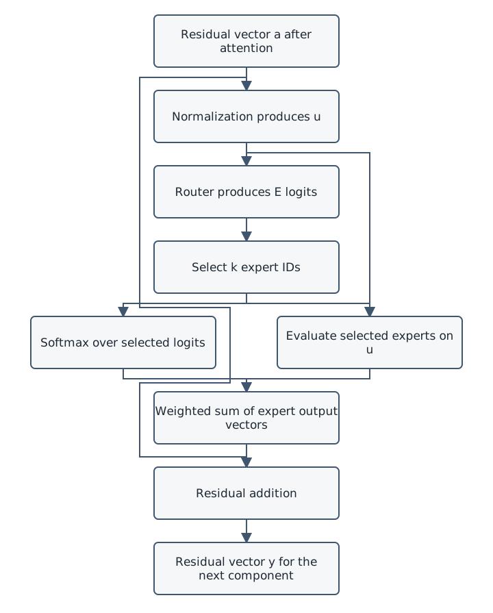
Original course diagram. The router determines both which expert functions run and how their output vectors are weighted. The bypass carries the unnormalized residual vector in this pre-norm example.
Not every MoE uses this exact weighting rule. In particular, keeping selected entries of a full softmax without renormalization gives a different update. A top-1 selected-only softmax produces coefficient one; Switch Transformer instead retains the winning full-softmax probability. Read the forward rule rather than inferring it from “top-\(k\).” Fedus et al., Section 2.1
A complete four-expert calculation
Consider a hand-constructed branch with \(d=2\), \(E=4\), and \(k=2\). To isolate routing, omit normalization and attention: the branch input and residual vector are both
\[ u=a=\begin{bmatrix}1\\1\end{bmatrix}. \]
Use an affine router with zero bias and
\[ W_r=\begin{bmatrix} \ln4&0\\ 0&\ln3\\ \ln2&0\\ 0&0 \end{bmatrix}. \]
Define four linear expert functions:
\[ f_0(u)=\begin{bmatrix}2u_1\\0\end{bmatrix},\quad f_1(u)=\begin{bmatrix}0\\3u_2\end{bmatrix},\quad f_2(u)=\begin{bmatrix}-u_1\\u_2\end{bmatrix},\quad f_3(u)=\begin{bmatrix}u_2\\u_1\end{bmatrix}. \]
These deliberately simple functions replace full nonlinear MLPs. They are invented arithmetic objects, not trained experts or simplified measurements from gpt-oss. Coordinates are numbered 1 and 2 in the equations; experts are numbered 0 through 3. If logits tie, prefer the smaller expert ID. That tie rule is part of this toy’s specification, not a claim about every library.
The router calculation gives
\[ z=[\ln4,\ln3,\ln2,0]^\mathsf T, \]
so exponentiation yields \([4,3,2,1]\) and
\[ p=[4/10,3/10,2/10,1/10]^\mathsf T. \]
Experts 0 and 1 rank highest. Their original probability mass totals \(7/10\), so the selected-only coefficients are
\[ \alpha=[4/7,3/7,0,0]^\mathsf T. \]
Only the selected expert outputs are needed:
\[ f_0(u)=[2,0]^\mathsf T,\qquad f_1(u)=[0,3]^\mathsf T. \]
Therefore
\[ m=\frac47\begin{bmatrix}2\\0\end{bmatrix} +\frac37\begin{bmatrix}0\\3\end{bmatrix} =\begin{bmatrix}8/7\\9/7\end{bmatrix}, \qquad y=\begin{bmatrix}15/7\\16/7\end{bmatrix}. \]
The larger gate belongs to expert 0, yet expert 1 makes the larger contribution norm here: \(9/7\) rather than \(8/7\). A routing coefficient and an output contribution are different measurements. Even contribution magnitude would not establish downstream importance, because later computations can amplify, suppress, or cancel directions.
Suppose we accidentally retain \(4/10\) and \(3/10\) as the combining coefficients. Then \(m=[4/5,9/10]^\mathsf T\) and \(y=[9/5,19/10]^\mathsf T\). Selection is unchanged, but the update has been scaled down. A log containing only the selected IDs would fail to expose this error.
Keep \(u\) and every expert fixed. Predict the update if you:
- add the same constant to all four router logits;
- increase expert 3’s logit from \(0\) to \(\ln(3/2)\);
- prohibit expert 0, choose the best two remaining experts, and renormalize;
- keep the original route and weights but replace expert 0’s output with zero.
The first two leave \(m\) unchanged under our rule. In the second case, the full distribution \(p\) changes, but the selected logits and their normalized coefficients do not. The third gives \(m=[-2/5,11/5]^\mathsf T\); the fourth gives \(m=[0,9/7]^\mathsf T\). Prohibiting a route and zeroing a contribution are different interventions.
Begin Trace and Perturb Expert Routing. Compute the toy router by hand, then extend the trace across positions and two small layers. The core needs no trained model, account, API, GPU, or paid compute. Return to its configuration inspection after the next section.
The gpt-oss specimen
Our concrete specimen is OpenAI’s gpt-oss-20b release, with gpt-oss-120b as a comparison. These are fixed documented designs, not recommendations about whichever model is newest.
The model card, version 1, Table 1 and Section 2.2 reports:
| Model | Layers | Experts per MoE layer | Selected per token per layer | Total parameters | Active parameters |
|---|---|---|---|---|---|
| gpt-oss-20b | 24 | 32 | 4 | 20.91 billion | 3.61 billion |
| gpt-oss-120b | 36 | 128 | 4 | 116.83 billion | 5.13 billion |
Counts in billions are the card’s rounded figures. Its active-count convention includes unembedding parameters but excludes embeddings. Both models use pre-branch RMSNorm and selected-only softmax weighting. The count of experts is per layer, not one shared bank for the entire network.
The 20b configuration pinned to revision f81fef1ddd90d214968e951a76834f1ded130a18 records hidden_size: 2880, intermediate_size: 2880, num_hidden_layers: 24, num_local_experts: 32, and num_experts_per_tok: 4. It also contains experts_per_token: 4. Names depend on the configuration format; do not silently substitute a familiar field from another model.
Read that JSON beside OpenAI’s reference MLPBlock, pinned to commit 243a1b02767da73bd2e3975be250afa801635866. The forward method normalizes the input, projects router logits, selects experts, applies softmax to their selected logits, evaluates the corresponding expert parameters, combines their outputs, and adds the residual. Its expert nonlinearity is a particular clamped SwiGLU variant. Our linear toy reproduces the routing arithmetic, not that expert computation.
A configuration describes dimensions and settings. It does not contain learned router weights, expert weights, or the activations for your prompt. Reading output_router_logits: false tells you a stored default, not whether a particular service can expose routing. The reference source establishes a computation; tracing an actual trained run additionally requires compatible weights and an instrumented runtime.
Count parameters before estimating memory
Suppose an invented network contains \(P_s\) always-used parameters and \(L\) routed layers, each with \(E\) distinct equal-sized experts of \(P_e\) parameters. Put router parameters in \(P_s\). Under a deliberately simplified accounting convention,
\[ P_{\mathrm{total}}=P_s+LEP_e,\qquad P_{\mathrm{active}}=P_s+LkP_e. \]
For \(P_s=100\), \(L=2\), \(E=4\), \(P_e=10\), and \(k=2\), the counts are 180 total and 140 active. Multiplying the total by \(k/E\) would incorrectly give 90, because it would sparsify the always-used part too. Embedding lookups and tied weights require explicit counting conventions in real networks.
A gated expert with three weight matrices of sizes \(m\times d\), \(m\times d\), and \(d\times m\) has \(3dm\) matrix coefficients. Ignoring biases and all other components, the 20b dimensions imply
\[ 24\times32\times3\times2880^2 =19{,}110{,}297{,}600 \]
stored expert-matrix coefficients, versus
\[ 24\times4\times3\times2880^2 =2{,}388{,}787{,}200 \]
used along one token’s selected expert path. These are our dimension-based calculations, not a replacement for the whole-model counts. Attention, routers, normalization, biases, and the output projection still matter.
The other distinction is memory residency. Unselected experts do not disappear. A runtime must have their weights available when subsequent tokens need them. They may all reside on one accelerator, be distributed across devices, or be moved from another memory tier. Different tokens in a batch can collectively activate many more than \(k\) experts in a layer.
A raw weight-storage estimate uses the stored parameter arrays and their representations. A runtime estimate must additionally include quantization metadata, caches, activations, temporary buffers, allocation overhead, and possibly duplicated or converted weights. Training adds gradients and optimizer state. Neither estimate is simply “active parameters times bytes per number.”
For example, the gpt-oss card reports quantized checkpoints of 12.8 GiB for 20b and 60.8 GiB for 120b. Checkpoint size does not guarantee runtime memory fit. Model card, Table 1 and Section 2.1
Sparse expert execution can reduce arithmetic relative to executing every expert, but arithmetic is not latency. Routing, token dispatch, memory movement, small expert batches, and cross-device communication all consume time. Actual speed needs a measured workload and runtime.
A fresh route at each position and layer
A router ordinarily reads the current hidden representation at a particular layer. Earlier attention may already have mixed information from other positions into it. Consequently, two occurrences of the same token ID can follow different routes when their contexts differ.
A token can also choose different experts at different depths. Expert 7 in layer 2 is not automatically the same function as expert 7 in layer 17. Treat the pair (layer, expert ID) as the component’s address. Changing one early route can alter later hidden states and therefore later routing decisions.
In a decoder model, routing occurs while processing prompt positions and while processing generated positions. It is not reserved for the visible answer. A run log should identify sequence position and whether the measurement belongs to prompt processing or a generation step. With caching, the runtime need not recompute every old position at every generation step.
Now return to the course’s recurring question: where does this behavior live? The router’s learned projection lives in model weights; the selection and combination rules live in its architecture and implementation; the vector being routed depends on the input context and previous computation. An application choosing between two whole language models is a separate, outer routing decision. A product’s “automatic model” option tells us nothing by itself about whether either chosen model contains MoE layers.
Learning routes and keeping experts useful
During training, the model’s objective supplies feedback to the parameters involved in its computation. Selected expert functions can receive gradients through their outputs. The router can receive gradients through the selected combining coefficients, within regions where the selected set remains unchanged. The discrete membership decision itself is not an ordinary smooth operation.
This creates a useful boundary case. For selected-only normalization with \(k=1\), the sole coefficient is identically one. Its local derivative with respect to the selected logit is zero. Training a router in that situation needs another learning signal or a different gate rule; one cannot assume that every top-1 scheme trains exactly like our top-2 formula. Shazeer and colleagues discuss differentiable gate values for \(k>1\) and use additional routing mechanisms in their system. Shazeer et al., Section 2.1
Ordinary inference uses the learned parameters without optimizing them. Selecting an expert is not retraining it, and a different route is not evidence that new knowledge was permanently stored. Module 3 will develop the training process more fully.
Routing also determines how much work reaches each expert. Imagine twelve token representations, each selecting two experts from a bank of four. There are 24 assignments. Counts of \([6,6,6,6]\) and \([12,12,0,0]\) obey the same top-2 rule, yet distribute computation and training examples very differently.
Assignment counts measure work allocations. Summed probabilities or combining coefficients measure a different quantity: a selected expert with a small coefficient still has to run. Keep those measurements separate.
Load balancing concerns the distribution of work. Some systems use auxiliary training losses to discourage concentrated routing; the exact loss, measurement unit, and trade-off vary. Switch Transformer supplies a concrete example with an auxiliary balancing loss and a fixed per-expert capacity. When its capacity overflows, a token can skip the expert computation while continuing through the residual path. “Dropped” in this setting does not mean deleting the token from the input text. Fedus et al., Section 2.2
Capacity limits and dropping are not defining requirements of MoE. MegaBlocks develops block-sparse computation that accommodates uneven assignment counts without dropping tokens. This is an implementation alternative to a particular capacity trade-off, not proof that routing imbalance has no cost. Gale et al., Sections 2–4
What makes an expert an expert
The name is suggestive, but no step in our router equation assigns a network the job “mathematician,” “poet,” or “fact checker.” Expert parameters and routing patterns are learned under the training setup. The architecture alone guarantees neither predefined roles nor a neat division into semantic domains.
Empirical specialization is a question to investigate. In its analysis of selected layers and datasets, the Mixtral paper found little clear topic-based separation and described routing patterns associated with syntax and token locality. That is evidence about the studied model and samples, not a theorem that experts can never specialize by topic. Jiang et al., Section 5
Suppose a trace selects one expert frequently in code prompts. Plausible explanations include punctuation, indentation, token identity, sequence position, or a broader feature of the hidden representation. Calling it “the coding expert” outruns the measurement. Compare matched inputs, distinguish layers, inspect output contributions, and test held-out cases before making a stronger claim.
Interventions require equal care. Prohibiting an expert, changing a logit, replacing an output with zero, and forcing an arbitrary expert set alter different computations. Forced routing can send a representation through a function that was rarely trained on such inputs. A performance drop can demonstrate sensitivity to the intervention without revealing a clean human-readable function. Use a baseline, state the exact intervention boundary, and separate immediate effects from downstream changes.
Check your understanding
Answer without looking back, then check the reasoning below.
- What are the shapes of \(W_r\), \(z\), an expert output, and the combined update?
- Why can two implementations select identical experts but produce different residual updates?
- In the toy example, force the set \(\{2,3\}\) and renormalize their original logits. What are \(m\) and \(y\)?
- Does top-4 routing imply that only four expert parameter sets are stored, or that a batch uses only four?
- What does the gpt-oss-20b configuration establish that a routing trace does not, and vice versa?
- Why is a routing-frequency plot insufficient to name an expert’s semantic role?
- With \(k\) fixed, does doubling \(E\) necessarily double per-token expert arithmetic? What still increases or might become harder?
- \(W_r\) is \(E\times d\), \(z\) has \(E\) entries, and both output vectors have \(d\) entries. We use column vectors for individual positions.
- They might use different combining coefficients, expert outputs, normalization, or residual boundaries. Selected IDs alone do not specify the computation.
- The coefficients are \(2/3\) and \(1/3\). Thus \(m=[-1/3,1]^\mathsf T\) and \(y=[2/3,2]^\mathsf T\).
- Neither. Selection is per token per routed layer. Other expert weights remain part of the model, and other tokens can select them.
- The config states architectural dimensions and stored settings. A correctly instrumented trace establishes actual selected routes and values for one specified execution. Neither alone explains why a trained expert performs its function.
- Frequency establishes an association with sampled inputs. Tokenization, position, and other features can explain it; a functional claim needs better controls and evidence.
- Not for fixed-size experts with the same \(k\). Stored expert parameters increase, the router has more candidates to score, and memory movement, dispatch, or load balancing can become harder. Whole-runtime cost is not fixed by the expert arithmetic alone.
More Learning
- gpt-oss Model Card — OpenAI, version 1. Read Table 1 and Section 2.2. Check the active-parameter footnote before comparing the two model names.
- gpt-oss reference forward computation — OpenAI, pinned commit. Match each operation in
MLPBlock.forwardto this lesson’s diagram. Notice where the residual addition occurs. - Outrageously Large Neural Networks — Shazeer et al.. Read Section 2 for sparse gating and Section 4 for balancing. Separate the paper’s noisy training rule from our deterministic toy.
- Switch Transformers — Fedus et al.. Compare its top-1 gate, capacity handling, and balancing objective with our selected-only top-2 rule.
- Mixtral of Experts — Jiang et al.. Read Section 5 as an example of testing a specialization hypothesis. Identify the sampled layers and datasets before generalizing.
- MegaBlocks — Gale et al.. Optional systems reading. Trace how grouping and ungrouping token representations connects the mathematical mixture to efficient execution.
We have now assembled the main architectural pieces. Module 3 asks how training selects the weights that make these computations useful.