4.1 — Inference: Running a Trained Model

Module 4 — Running Models and Turning Them into Systems

A checkpoint becomes a running computation

Training leaves an artifact. Inference turns that artifact and an input into model outputs. Between the two sit loading code, numerical formats, memory allocation, token selection, and a runtime that decides which operations happen when. These choices can change speed, resource use, and generated text even when the learned weights have not been updated.

This lesson follows one request from files to tokens. The recurring question is where does the behavior live? A different tokenizer, sampling rule, cache policy, or hardware kernel is a different intervention. Calling all of them “changing the model” hides the mechanism you need to understand.

By the end, you should be able to:

• distinguish checkpoint loading, a forward pass, and autoregressive generation;
• explain prefill and decode without confusing cached activations with learned weights;
• read precision claims separately for storage, arithmetic, and accumulation;
• budget runtime memory beyond the weight file;
• calculate temperature and nucleus sampling on a small distribution;
• design a fair, reproducible comparison of inference settings.

NoteMath to know / refresh

Needed now: probability distributions, logarithms, powers, units, and finite numerical representation.

Useful refresh: softmax turns logits into probabilities; dividing a logit by temperature changes relative odds. A byte is eight bits, a decimal MB is \(10^6\) bytes, and a MiB is \(2^{20}\) bytes.

Side trail: rounding-error analysis, matrix-multiplication kernels, and queueing theory. Their full derivations are unnecessary for this lesson.

Load a compatible set of artifacts

An inference checkpoint normally needs more than a weight file. The runtime needs an architecture implementation and its configuration: dimensions, block count, attention layout, normalization, positional mechanisms, and other choices determining how tensors are used. The tokenizer supplies the mapping between text and token IDs. Special-token rules and, for chat models, the serialization template determine the actual sequence supplied to the network.

An inference engine coordinates execution: it selects kernels, manages memory and caches, and may batch or schedule requests. A high-level generation library can provide a simple runtime; a serving engine adds machinery for many concurrent requests. Neither label identifies a new set of trained weights.

A configuration alone does not contain trained weights. Conversely, a collection of weight tensors cannot explain its own architecture reliably. Shapes help detect incompatibility, but matching dimensions do not prove that a tokenizer assigns the intended meaning to each embedding row. Preserve the compatible bundle and its revision.

A loader may read checkpoint shards, construct modules, convert tensor formats, place tensors on devices, and report missing or unexpected keys. A loading override can differ from configuration metadata. Transformers exposes explicit revision, local-file, safetensors, dtype, and attention-implementation options; its versioned documentation describes their meanings. Unexpected loading warnings deserve investigation rather than automatic suppression. Transformers model-loading reference

Our small specimen is EleutherAI/Pythia-14M at revision 94f7c35d5e9f2e9bac8ca839329f505b4d007d5d, the same bounded artifact used in Lab 05. Its configuration describes six GPT-NeoX blocks, residual width 128, four attention heads, and a configured maximum sequence length of 2,048 positions. Its safetensors weight file is 28,143,920 bytes; tokenizer and configuration files add to the download. This tiny base model is useful for inspecting mechanics. Its continuation quality is not representative evidence about contemporary assistants. Pinned publisher commit

Separate setup from execution. Downloading an artifact, loading it into memory, and answering with an already loaded model are three different activities. A “first response” measured across all three answers a different question from warm inference latency.

A forward pass is one component of generation

For an ordinary decoder-only language model, a forward call receives token IDs, an attention mask, positional information, and optionally a cache. A full-prefix call commonly returns logits shaped \((B,S,V)\): batch size, sequence length, and vocabulary size. The last relevant position provides scores for the next token. Earlier positions also contain predictions, conditioned only on their permitted prefixes.

The forward call does not by itself decide how long to continue. A generation loop selects a token, appends it, prepares the next input, repeats the model computation, and checks stopping conditions. An end token, a token budget, and an application stop string are different stopping mechanisms. Some engines avoid materializing logits for every prompt position when only the final one is needed. Verify the returned interface rather than assuming every runtime stores the same intermediates. GPT-NeoX model interface

For inference, evaluation mode and disabled gradient tracking address different concerns. model.eval() changes the behavior of modules such as dropout. torch.inference_mode() removes autograd-related overhead but does not, by itself, select evaluation mode. Neither instruction chooses greedy decoding or fixes a random seed. PyTorch evaluation-mode explanation

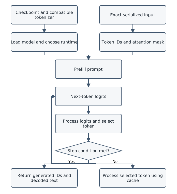
Original course diagram. Prefill calculates the prompt’s states and its next-token scores. Selection happens outside that forward computation. In the cached path, each subsequent model call processes the previously selected token. The diagram omits batching and scheduling so the dependencies remain visible.

Prefill and decode have different workloads

During prefill, the model processes the prompt and prepares the state needed to continue. During decode, ordinary autoregressive generation repeatedly processes newly selected tokens. The first output token can be selected from prefill’s final logits; generating \(N\) output tokens then requires \(N-1\) further forward calls, assuming no extra verification or speculative steps.

A KV cache retains prior attention keys and values. Correct incremental decoding reuses these activations instead of rerunning the entire prefix through each layer. It still computes the new token’s projections and MLP updates, and global attention still reads a growing history. Cache entries belong to particular inputs, weights, masks, and positions. They are not training updates or a general-purpose store of facts. Transformers caching explanation

The architecture and cache-size derivation appeared in Lesson 2.4. Here the operational distinction matters: a correct cache should preserve the intended mathematical computation while changing how much work is repeated. Cached and uncached floating-point results need not be bit-for-bit identical. Compare them on identical prefixes before attributing a difference in generated text to a broken cache.

Large prompt matrices can exploit parallel arithmetic differently from a single sequence’s one-token decode. At small batches, decode can be constrained by moving weights and cache data through memory rather than by peak arithmetic capacity. These are workload-dependent tendencies, not universal classifications. A tiny CPU model may spend a substantial fraction of its time in dispatch, allocation, and Python overhead. It cannot establish the bottleneck of a large accelerator deployment. NVIDIA inference-performance guide

Numerical precision has several meanings

When a model is described as “BF16” or “four-bit,” ask which part of the computation that describes:

1. Stored weights: values in the checkpoint or runtime weight representation.
2. Activations and cache: intermediate tensors produced for the current input.
3. Arithmetic operands: representations actually consumed by a kernel.
4. Accumulation: the format used while adding many products.
5. Returned results: the representation after casting or rounding.

These need not match. A matrix multiplication can consume low-precision operands, accumulate in a wider format, and return a lower-precision tensor. Wider accumulation reduces one source of numerical error; it does not recover information already lost when the operands were quantized. A tensor’s reported dtype alone does not fully specify the hardware arithmetic. PyTorch numerical-accuracy notes

Format	Bits per scalar	Main distinction
FP32	32	Eight exponent bits and 23 explicit fraction bits
FP16	16	Five exponent bits and ten explicit fraction bits
BF16	16	Eight exponent bits and seven explicit fraction bits
FP8	8	A family of encodings and scaling recipes
Four-bit representation	4 before overhead	Could be integer, floating-point, or a codebook index

The sign consumes another bit in the three conventional floating-point rows. NVIDIA format reference Exponent bits largely determine range; fraction bits determine spacing within a range. BF16 has FP32-like exponent range but much coarser precision. FP16 has finer spacing than BF16 near one but a narrower range. Equal file size therefore does not imply interchangeable numerical behavior. Google Cloud explanation of BF16

For normalized numbers in \([1,2)\), the adjacent-value spacing is \(2^{-23}\) for FP32, \(2^{-10}\) for FP16, and \(2^{-7}\) for BF16. Thus FP16’s spacing there is \(1/1024\), whereas BF16’s is \(1/128\). This is a local spacing calculation, not a global error bound. Larger magnitudes have larger absolute spacing; overflow, underflow, and subnormal handling are separate issues.

FP8 is not a single numerical contract. E4M3 and E5M2 allocate different numbers of exponent and fraction bits; special-value conventions and scaling also matter. A method can scale a tensor or block before conversion to use the limited representable range effectively. “Supports FP8” must be followed by questions about the exact encoding, scale granularity, supported operations, and kernel implementation. FP8 Formats for Deep Learning

Likewise, a four-bit code need not represent an ordinary four-bit integer. NF4, for example, uses a particular nonuniform codebook developed for quantized neural-network weights. This is different from simply casting every tensor to a universal FP4 type. Methods also differ in calibration, grouping, outlier handling, and which parameters remain at higher precision. QLoRA paper

Weight-storage format and compute dtype can be configured separately in concrete quantization libraries. Scales, other metadata, and unquantized modules consume additional memory; cache quantization is a separate choice. Whether a compressed representation runs faster depends on conversion costs and hardware support as well as fewer bytes moved. The CPU lab uses FP32 to keep its experiment interpretable, not because FP32 is always the fastest format. Transformers bitsandbytes documentation

Budget for a running request

A useful first budget is

\[ M_{\mathrm{runtime}}\approx M_{\mathrm{weights}}+M_{\mathrm{KV}}+ M_{\mathrm{live\ activations}}+M_{\mathrm{workspace}}+ M_{\mathrm{other}}. \]

This is an accounting framework, not an exact allocator equation. Some categories overlap in time or share storage. Peak use matters: loading can temporarily hold multiple representations, and prefill’s peak can differ from decode’s. Distinguish live tensor bytes, allocator-reserved memory, process memory, and whole-device memory. CPU RAM and accelerator memory may each require a separate budget.

Consider an invented 8-GiB device budget: 4 GiB for resident weights, 1.5 GiB for cache, 0.75 GiB for peak activations, 0.5 GiB for workspace, and 0.5 GiB for other runtime use. The sum is 7.25 GiB, leaving 0.75 GiB. This margin is not a guarantee against an out-of-memory error; the categories are estimates and their peaks may have been missed. “The weights fit” would have ignored almost half the proposed use.

Even a packed-weight estimate needs overhead. Suppose exactly \(2^{20}\) weights use four-bit codes and one two-byte scale per group of 64 weights. The codes occupy 0.5 MiB, and the scales add

\[ \frac{2^{20}}{64}\times2=32{,}768\text{ bytes}=0.03125\text{ MiB}. \]

Total: 0.53125 MiB before alignment, metadata, or any other tensors. These are original bookkeeping examples, not measured model footprints.

The cache can become a major variable as simultaneous requests and sequence lengths grow. Allocation strategy matters alongside logical tensor size: unused reserved slots and fragmentation can reduce the useful batch capacity. PagedAttention addresses this serving problem using block-based KV memory management. It does not erase the underlying need to represent retained states. PagedAttention paper

Batching introduces bookkeeping as well as parallelism

A static batch groups several sequences into one operation. The weights can be shared across the batch, while each sequence needs its own logical context and generation state. In a rectangular padded batch, shorter inputs occupy some unused token positions. An attention mask tells the model which positions are padding; it does not automatically make every kernel skip the associated work.

Generation also needs scores from the correct final input position. The familiar decoder-only Transformers generation path expects left padding for mixed-length inputs because it selects from the final sequence position. Right padding with a mask is not enough to fix that selection rule. This is a runtime convention, not a claim that causal Transformers can never handle right-padded data. Transformers generation tutorial

Keep request IDs when sorting by length or changing batch order. Otherwise an apparently valid answer can be attached to the wrong request. Record masks and position handling too. Batched kernels and singleton kernels can produce small numerical differences, and a shared random stream can assign different draws when row order changes.

Serving systems may use continuous batching, admitting new requests as others finish rather than waiting for one fixed group to complete. This can improve resource use but adds scheduling choices. Higher aggregate throughput does not imply lower latency for each person, especially if forming batches introduces waiting. A benchmark must say whether it measures one request, a fixed batch, or a loaded service. Orca serving paper

From logits to a sampling distribution

Let \(z_i\) be the next-token logit for vocabulary item \(i\). At positive temperature \(T\),

\[ p_i(T)=\frac{\exp(z_i/T)}{\sum_j\exp(z_j/T)}. \]

For numerical stability, subtract the largest scaled logit before exponentiating; this leaves the distribution unchanged. Lower positive temperature sharpens relative odds, and higher temperature flattens them. For two tokens,

\[ \frac{p_i(T)}{p_j(T)}=\exp\!\left(\frac{z_i-z_j}{T}\right). \]

Temperature preserves logit ranking when \(T>0\). It changes probabilities, not which token is largest. Greedy decoding selects a maximum-scoring token without sampling; setting do_sample=False is clearer than treating the undefined division by \(T=0\) as an ordinary softmax operation.

Top-k keeps a specified number of highest-scoring candidates, subject to an implementation’s tie policy. Top-p, or nucleus sampling, selects a high-probability set whose cumulative mass reaches a threshold, then renormalizes over the retained set. The number retained can vary from one position to the next. The original nucleus-sampling paper studied how truncating the unreliable tail affected open-ended text generation; it did not turn next-token probability into a factuality score. Holtzman et al.

An exact example with an explicit cutoff

Invent a four-token vocabulary \(A,B,C,D\) with logits

\[ z=(\log8,\log4,\log2,\log1). \]

These are teaching values, not measured Pythia logits. At \(T=1\), exponentiation gives \((8,4,2,1)\) and

\[ p=(8,4,2,1)/15. \]

Greedy decoding chooses \(A\). Sampling can choose any of the four. Top-k with \(k=2\) retains \(A,B\) and produces probabilities \((2/3,1/3,0,0)\).

For this example, define top-p precisely: sort by descending probability, resolve ties by token order, and retain the smallest nonempty prefix whose cumulative mass is at least the threshold. Keep the token that reaches or crosses it. At \(p=3/4\), \(A\) alone has \(8/15<3/4\); \(A,B\) have \(12/15>3/4\). Retain \(A,B\). At the exact boundary \(p=4/5\), the same two tokens suffice because \(12/15=4/5\).

Now set \(T=1/2\). Dividing logits by one-half squares their exponentials:

\[ p(1/2)=(64,16,4,1)/85. \]

Apply top-p with threshold \(3/4\) afterward. Since \(64/85\approx0.752941>0.75\), only \(A\) survives. Sampling now returns \(A\) with probability one.

Order changes the answer. If we first select the \(T=1\) nucleus \(\{A,B\}\) and then apply \(T=1/2\) only to those retained logits, their probabilities become \((64/80,16/80)=(4/5,1/5)\). Token \(B\) remains possible. Temperature-then-nucleus and nucleus-then-temperature are different algorithms.

An implementation may use an equivalent ascending-tail removal procedure, impose a minimum candidate count, or encounter floating-point differences near an exact cutoff. Inspect its boundary rule. The pinned Transformers source makes its masking and minimum-token behavior explicit. Do not interpret a one-token boundary discrepancy as a new property of the trained weights. Logits-processing source

Reproducibility is a complete experimental specification

Generation may also apply repetition penalties, token bans, minimum-length constraints, or other logit processors. These transformations can alter rankings or support before selection. Record their order and effective values, not just temperature and top-p. In particular, a library default for top-k can quietly make an intended “top-p only” experiment a combined filter. Generation configuration reference

A seed controls a pseudorandom sequence within a particular implementation. It does not guarantee the same continuation across package versions, devices, batching arrangements, or numerical kernels. Greedy decoding removes sampling randomness, but a tiny numerical change can still reverse nearly tied logits. Once a different token is chosen, all later prefixes differ. Record the first divergence rather than treating the rest of the output as independent discrepancies. PyTorch reproducibility notes

Most importantly, the sampling distribution describes token selection under the model and runtime. It is not a probability that a whole answer is true. Lower temperature can make an error repeatable. Higher temperature can reveal alternatives, but it does not supply missing evidence. Evaluate a factual claim using appropriate external evidence and evaluate task performance using a declared task and rubric.

Measure what a person or system actually waits for

Define timing boundaries before collecting numbers:

• Time to first token, or TTFT: elapsed time from the chosen request start to availability of the first output token. A service measurement can include queueing, transport, and preprocessing.
• Inter-token latency: time between successive output tokens, excluding the wait for the first. Streaming chunks need not correspond one-to-one with tokens.
• Request latency: elapsed time until the requested response completes.
• Output-token throughput: total output tokens divided by the declared wall-clock interval, across the declared workload.

A local prefill-only timer is useful, but it is not automatically service TTFT. Input-token throughput and output-token throughput also count different work. NVIDIA metric definitions

For one local request with \(N>1\) output tokens, an average post-first-token interval is \((t_N-t_1)/(N-1)\). It cannot be inferred accurately by dividing total request time by \(N\) when prefill is substantial. If \(N=1\), report the inter-token metric as unavailable.

Separate download, loading, warmup, tokenization, model execution, sampling, and text decoding where the question requires it. Repeat measured runs and retain their spread; report a median rather than presenting the fastest run as typical. Hold hardware, thread count, prompt IDs, actual output length, cache policy, and timing boundaries fixed when comparing an optimization. Synchronize asynchronous accelerators around appropriate measurement boundaries. PyTorch benchmarking guide

A change in sampling settings can change when an end token appears. A shorter response may finish sooner without any faster token computation. Likewise, caching can help a longer workload while showing little benefit on a tiny one. The lab asks you to preserve all outcomes and explain the workload before naming a winner.

TipLab recommended here

Lab 12 — Measure Inference and Sampling reuses the bounded Pythia artifact on CPU. Compare greedy and seeded sampling, check cached and uncached logits on identical prefixes, and measure repeated fixed-workload runs. No API, account, accelerator, or paid service is required.

Retrieve and predict

1. Why can changing the tokenizer break a run even if the embedding dimensions still match?
2. After prefill, how many additional ordinary forward calls select a total of eight output tokens?
3. Does loading FP16 checkpoint values into FP32 recover precision lost before saving?
4. In the four-token example, what survives \(T=1/2\) followed by top-p \(=3/4\)? What survives the opposite order?
5. Why should a cache correctness test supply identical next-token prefixes to both paths?
6. A faster run produced half as many output tokens. What remains unknown?
7. Predict whether batching three requests will necessarily make every request finish sooner. Explain.

NoteAnswers and reasoning

1. Token IDs may refer to different text units. Compatible shapes cannot establish compatible semantics or serialization.
2. Seven: prefill already supplies the first choice’s logits.
3. No. FP32 can represent the saved values more widely, but cannot reconstruct discarded information.
4. Temperature first leaves only \(A\). Nucleus first retains \(A,B\), subsequently sampled with probabilities \(4/5,1/5\).
5. Different prefixes represent different mathematical questions. After divergence, comparing free-running logits no longer isolates caching.
6. Whether the runtime processed equivalent work faster. Compare actual lengths and separately defined latency or throughput.
7. No. Shared computation may improve aggregate throughput, while padding, scheduling, or contention can increase individual latency.

More Learning

1. Transformers generation configuration, v4.57.1. Read the distinction between selection, stopping, cache, and returned-output settings. This pinned interface is a reference, not an instruction to install an old release without checking compatibility.
2. The Curious Case of Neural Text Degeneration. Read the motivation for nucleus sampling and distinguish its open-ended generation evaluation from factual correctness.
3. PyTorch numerical accuracy. Follow the examples explaining why mathematically equivalent execution paths can differ numerically.
4. FP8 Formats for Deep Learning. Compare E4M3 and E5M2 and identify which properties a label such as “FP8 inference” leaves unspecified.
5. Efficient Memory Management for Large Language Model Serving with PagedAttention. Connect logical cache contents to allocation and serving capacity.
6. PyTorch benchmarking guide. Study warmup, repetitions, thread count, and synchronization before making speed claims.

Download Markdown · PDF — Letter · PDF — A4

← Previous · All lessons · Next →