6.1 — Experimental Design for LLM Labs

Module 6 — Experimental Methods and Integration

Make the comparison answer the question

An intervention changes a model’s output. A new prompt gets more answers right. A second attempt succeeds where the first failed. Each observation can be useful, but none explains itself. Perhaps the intervention altered an irrelevant feature, the new prompt received easier questions, or the second attempt benefited from information the first never saw.

Experimental design connects a question to a comparison that could answer it. It starts before the interesting output appears. You decide what changes, what stays fixed, what counts as evidence, and which alternative explanations the comparison can address. Careful analysis cannot recover information that an unsuitable comparison never collected.

Earlier Labs already used pieces of this discipline: shared candidate streams in Lab 4.2, observation checks in Lab 5.1, separate fitting and evaluation data in Lab 5.2, and frozen intervention predictions in Lab 5.3. This lesson brings those choices together. The goal is a small, interpretable instructional experiment, not a claim that one exercise establishes a new scientific result.

By the end, you should be able to:

turn a vague claim into a falsifiable comparison;
identify variables, controls, confounders, and the relevant independent units;
preserve pairing, separate exploration from confirmation, and avoid test leakage;
calculate a paired effect and explain an uncertainty interval’s assumptions;
report small, negative, and inconclusive results without hiding failures.

Math to know / refresh

Needed now: a mean averages values; variance measures their spread; a distribution describes possible values and their probabilities. An effect size describes the magnitude of a difference. A confidence interval comes from an uncertainty procedure with assumptions.

Useful refresh: hypothesis tests, multiple comparisons, and regression adjustment.

Side trail: hierarchical models, equivalence testing, sequential designs, and causal inference. We will recognize where these methods are needed without pretending to implement them all.

Turn an attractive claim into a vulnerable one

“More reasoning makes the model better” leaves almost everything undecided. Which model? What counts as reasoning? Better at what? Compared with which resource budget? A claim that changes its meaning after every result cannot be tested fairly.

A narrower instructional hypothesis is: for one fixed checkpoint and a declared population of arithmetic task families, adding one fixed checking instruction increases mean rubric score by at least five points on a 0–100 scale, with no more than a quarter increase in the specified inference budget. The instruction, rubric, budget accounting, and task construction must be written down. These details are not administrative clutter; they define the claim.

A hypothesis is a proposed explanation or prediction. Its operational version specifies measurements that could count against it. Falsification means exposing it to such a possibility. A worse score challenges the prediction. An interval too wide to distinguish a meaningful benefit from no benefit leaves the question unresolved. Neither outcome licenses changing “arithmetic” to “creative writing” after seeing which category looks favorable.

Distinguish a claim about this particular dataset from one about a larger population. The average of eight fixed task families is an exactly defined descriptive quantity. The average over future task families is an unknown population quantity, often called an estimand. Its interpretation depends on how those eight families represent the intended population. A convenience sample does not become representative because its arithmetic is precise.

Record a prediction and a reason before analysis, including what would weaken your expectation. You can expect a gain of three points while testing a practical requirement of five. Your expectation, your acceptance threshold, and the eventual observation are three different objects.

Locate the independent and dependent variables

The independent variable, or factor, is what the experiment deliberately varies. In the example it is the presence of one particular checking instruction. Its two levels are control and treatment. The dependent variable, or outcome, is what you measure: the predefined rubric score. Latency, token use, and invalid-answer rate can be secondary outcomes.

Changing the model, prompt, decoding settings, and tool access together estimates the effect of a package. That may be the right product question, but it cannot isolate the instruction’s contribution. Conversely, holding every resource fixed can exclude part of the mechanism you wanted to study. If the instruction works by using additional tokens, a strict token cap asks a different question from allowing extra tokens and measuring their cost.

Specify the comparison’s purpose first. “Which system produces more correct answers within this budget?” and “What changes when this instruction is added?” deserve different controls. A single-factor experiment is often easiest to interpret initially. Later, a factorial design can investigate interactions, such as whether an instruction’s effect changes with decoding temperature. An interaction means the effect of one factor depends on another factor’s level; it is not automatically measurement noise.

Metrics also contain choices. A grader that rewards verbose explanations can favor longer answers without measuring correctness better. Define answer extraction, rubric anchors, ties, malformed outputs, and refusal handling in advance. If human scoring is used, hiding condition labels and randomizing presentation order can reduce expectation effects. A model grader is another measurement instrument whose errors require inspection.

Controls answer particular alternative explanations

A baseline describes the comparison you would otherwise use. A control condition tests a specific alternative explanation. They sometimes coincide, but a single baseline rarely answers every question.

In an activation experiment, an unmodified pass gives the baseline. A zero-dose intervention checks whether the hook machinery itself changes results. A matched-norm random direction asks whether a chosen direction does more than a similarly sized perturbation. An opposite-sign intervention checks a directional prediction. These controls address different possibilities; passing one does not imply passing the others.

A confounder changes with the condition and can also influence the outcome, making attribution ambiguous. Easier tasks assigned mostly to treatment confound a prompt comparison. Running the baseline before a software update and treatment afterward mixes the treatment with an environment change. A longer context that accidentally includes the answer changes much more than formatting.

Blocking groups comparable observations so conditions are compared within the same nuisance setting. Pairing both conditions on each task is one useful form. Randomizing run order can distribute time-related effects rather than systematically giving one condition the warm cache. Neither step guarantees removal of every source of bias. NIST’s randomized block design guide develops this distinction between the factor of interest and nuisance variation.

Here is an original diagram of a small paired design. Each family’s raw records remain together throughout analysis.

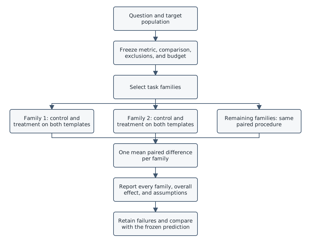
The diagram contains no arrow from a disappointing result back to quietly rewriting the prediction. A new idea can start a new, labeled exploratory analysis.

Count independent information rather than rows

The experimental unit is the unit to which a treatment can be independently assigned or applied. The sampling unit is the unit selected from a population. The analysis unit is what a statistical calculation treats as an independent contribution. These need not be identical, so name each rather than assuming “one row” settles the issue.

Imagine eight independently selected task families, each with two closely related wordings. You can apply both conditions to every wording, but the two wordings share content and difficulty. For a simple analysis aimed at new families, average the paired differences within each family and use eight family-level values. That estimates an equally weighted family average. Weighting every wording equally would target something different if families had unequal numbers of wordings.

Pseudoreplication treats related or duplicated observations as though they supply independent replication. Ten copies of one saved output are ten rows and one observation. Twenty tokens from one answer are not twenty independently sampled tasks. Several seeds on one checkpoint explore some inference variability, not variability across independently trained models.

Aggregation does not magically prove independence. Families can still share a source document or generation template. Several checkpoints may descend from the same training run. Identify the highest shared structure that matters to your claim. More complicated crossed structures, such as tasks evaluated under several independently trained checkpoints, may require a hierarchical analysis or separate summaries rather than one generic interval.

The distinction was visible in Lab 4.2: candidates inside a shared-failure request were dependent. More candidates did not create more independent requests. Likewise, repeating a deterministic forward pass checks reproducibility, but cannot create uncertainty about an unchanged output.

Pair tasks and describe what seeds accomplish

A paired comparison computes treatment minus control on the same unit. Difficult tasks can then be difficult for both conditions without obscuring the within-task change. Pairing can improve precision when the paired outcomes co-vary, but it must remain intact in the analysis. Computing uncertainty as if the groups were unrelated throws away that information. NIST’s treatment of paired observations introduces this correspondence.

For stochastic generation, declare how seeds are used. Reusing a seed can be a common-randomness strategy, but the same integer does not guarantee that two implementations consume matching random draws. Different token paths, sampling algorithms, or batching can break that correspondence. Save the procedure and actual outputs rather than claiming seeds make all comparisons equivalent.

Several fixed seeds are useful only when their role is clear. They might sample generation variability, initialization variability, or synthetic-data variability. They do not cover every source at once. Bouthillier and colleagues study how data sampling, initialization, and hyperparameter choices affect machine-learning comparisons; their result motivates recording the sources included and omitted, rather than relying on one favorable run. Accounting for Variance in Machine Learning Benchmarks

Template variants deserve similar care. Replacing a name in one question does not necessarily create an independent reasoning problem. Keep related variants identified and, when generalization to new templates is the question, separate entire template families across development and evaluation.

Give development and evaluation different jobs

A training set fits parameters. A validation set informs choices such as regularization, thresholds, prompts, intervention strength, or stopping. A test set evaluates the frozen choice. Those roles matter even when the base model is never trained: choosing a steering layer from its evaluation results is still selection.

For example, fit a probe and its normalization on training activations. Use validation families to choose a regularization setting. Then evaluate once on previously untouched test families. Recomputing normalization using the test distribution can leak information. Splitting nearly identical variants between training and test can measure familiarity with a template instead of generalization to another family. The validation approach is developed in An Introduction to Statistical Learning.

Exploratory work is where you discover patterns, inspect failures, change a rubric, and propose explanations. Confirmatory work evaluates a sufficiently specified plan against data that did not determine it. Both are useful. The problem is presenting a choice discovered through exploration as if it had been predicted independently.

A frozen plan should name the primary outcome, contrast, independent unit, sample size or stopping rule, exclusions, uncertainty method, and practical threshold. Save its timestamp and content hash. A hash helps detect later changes; it does not prove nobody previously saw the data. Be candid about prior exposure. Because this lesson prints its synthetic answers, the accompanying Lab rehearses pre-analysis discipline rather than creating genuinely unseen confirmatory evidence.

If a bug is found after testing, preserve the original run, document the correction, and rerun the corrected analysis under a new identifier. The repair can be necessary without retroactively making the first run valid.

Lab pause — Freeze the comparison before calculating

Open Lab 6.1 and complete Part 1. Read the fixture and uncertainty specifications in Parts 2–3 before doing their arithmetic: freeze the comparison, independent unit, practical threshold, predictions, and uncertainty assumptions first. Then return for the worked calculation. The answers are published here, so disclose any prior exposure; this rehearses pre-analysis discipline rather than creating unseen confirmatory evidence.

Work one paired calculation all the way through

Consider these original synthetic family-level scores. They are invented teaching data, not measurements of an LLM. In Lab 6.1, each family score is the mean of two correlated wording records.

Family	Control score	Treatment score	Paired difference
F01	50	54	4
F02	60	62	2
F03	55	61	6
F04	65	65	0
F05	70	74	4
F06	80	78	-2
F07	75	83	8
F08	85	87	2

Let \(d_i=y_{i,T}-y_{i,C}\). The mean paired difference is

\[ \bar d=\frac{1}{8}\sum_{i=1}^{8}d_i =\frac{24}{8}=3. \]

This is an effect size in original units: three rubric points. It is not three percent accuracy. The control and treatment means are \(67.5\) and \(70.5\), respectively. Their difference agrees with the mean of the differences because the pairing is complete and equally weighted.

The deviations from three are \([1,-1,3,-3,1,-5,5,-1]\). Their squares sum to \(72\). The sample variance and sample standard deviation of family differences are

\[ s_d^2=\frac{72}{8-1}=\frac{72}{7}, \qquad s_d=\sqrt{72/7}\approx3.2071. \]

Variance has squared-score units; standard deviation has score units. The spread describes differences between families, not uncertainty about a particular family’s recorded value. An optional standardized paired effect is \(d_z=\bar d/s_d\approx0.9354\). Its denominator is the standard deviation of paired differences. Do not silently compare it with an effect standardized using pooled unpaired scores.

A mean hides important structure. Six families improve, one is unchanged, and one worsens. Keep the whole table. Dropping F06 because it “did not respond” changes the question after observing the answer.

Attach uncertainty to an explicit model

For independent, identically distributed family differences, an estimated standard error of their mean is

\[ \operatorname{SE}(\bar d)=\frac{s_d}{\sqrt8} =\sqrt{\frac{9}{7}}\approx1.1339. \]

If these independent differences follow a normal population distribution, the usual two-sided 95% Student-\(t\) interval for the population mean is

\[ \bar d\pm t_{0.975,7}\operatorname{SE}(\bar d). \]

Using the rounded critical value \(2.365\) gives approximately \([0.3183,5.6817]\) score points. NIST explains the interval procedure and supplies the critical-value table.

Under its assumptions, the procedure with the exact critical quantile covers the fixed population mean in 95% of repeated samples; the rounded table value gives a close approximation. It does not assign a 95% probability to this particular fixed interval, and it does not describe where 95% of individual task effects lie. With only eight families, departures from the assumed distribution matter; a tidy-looking table cannot establish normality.

Here the scores were deliberately invented and families were not randomly sampled. The interval is therefore an illustration of a conditional calculation, not calibrated evidence about real tasks. The descriptive mean of the eight displayed families remains exactly three whether the population model is justified or not.

If resampling is used instead, resample whole paired families together. A bootstrap that independently resamples control and treatment, or treats related wordings as independent, answers a different question. A randomization test also needs a justified assignment or exchangeability model. Neither technique is an assumption-free way to manufacture certainty from arbitrary rows. Dror and colleagues discuss matching statistical procedures to NLP experiments and metrics. The Hitchhiker’s Guide to Testing Statistical Significance in Natural Language Processing

Separate statistical detection from practical meaning

Suppose the practical requirement was a gain of at least five points. The observed gain is three, and the illustrative interval includes effects below and above five. The data have not established the practical requirement. Even a statistically detectable departure from zero would not settle that decision.

A \(p\)-value is a probability, under the specified null model, of a test statistic at least as extreme as the observed statistic according to the chosen test. It is not the probability that the null hypothesis is true, the probability the treatment works, or a measure of effect magnitude. The American Statistical Association’s statement cautions against treating a threshold as a substitute for scientific reasoning.

Practical meaning can include cost and failures. A one-point improvement may be useful at unchanged cost. A five-point improvement may be unacceptable if it requires twenty times the resource budget or causes rare severe errors. State the relevant trade-off before seeing which outcome looks best.

An interval spanning important benefit and important harm is inconclusive for a decision. An interval concentrated near zero may rule out effects large enough to matter under the model and scope. “Not statistically significant” alone does not show equivalence. Formal equivalence claims require predefined margins and a suitable analysis.

Plan sample size and limit the search

Independent units generally improve precision more than duplicated records. Under the simple standard-error formula, quadrupling an independent sample approximately halves the standard error if variability stays similar. This is a planning approximation, not permission to multiply nominal rows while preserving the same few families.

Choose sample size using the smallest effect worth detecting, plausible variability, and resource limits. A pilot can inform those quantities, but searching for an optimistic pilot result undermines the plan. Power is the probability that a specified procedure detects a specified effect under its assumptions. Card and colleagues show why underpowered NLP comparisons can struggle to distinguish meaningful changes from noise. With Little Power Comes Great Responsibility

Testing many layers, prompts, metrics, and seeds creates many opportunities for a favorable accident. Under twenty independent true-null tests, each with a false-positive probability of \(0.05\), the probability of at least one false positive is \(1-0.95^{20}\approx0.642\). Dependence changes this calculation, but does not make selection harmless.

Predeclare a primary contrast and show the other analyses as diagnostics or exploration. For a specified family of \(m\) tests, Bonferroni’s method uses a per-test threshold of \(\alpha/m\) to bound the family-wise false-positive probability under valid individual tests; independence is not required. It can be conservative and does not repair leakage or confounding. NIST’s Bonferroni guide

Do not keep adding examples until a desired threshold is crossed. Sequential analysis is possible, but requires a procedure designed for repeated looks. A fixed stopping rule is simpler for these Labs.

Finish with an auditable result

Preserve configuration, model revision when relevant, data and code hashes, software versions, conditions, seeds, raw outcomes, exclusions, and error logs. Keep unsuccessful runs. Reproducibility includes knowing what did not complete and which conclusions depend on a failed check.

Use public or synthetic prompts for instructional exercises. Do not include private messages, credentials, or identifiable personal data merely to make a fixture realistic. Agree on any human evaluation and data-sharing arrangements before collecting responses. Set limits for runtime, storage, network access, and paid resources; stop when they are reached. A failed run does not silently authorize a larger model or cloud bill.

A useful conclusion reports what changed, by how much, under which conditions, and what remains uncertain. “This frozen comparison showed mixed family-level changes and did not establish our five-point requirement” can be a successful learning outcome. It gives the next question a firmer starting point.

Continue with Lab 6.1 — Design a Controlled Experiment. It uses only a tiny synthetic dataset and Python’s standard library, so the quality of the reasoning cannot be purchased with a larger compute budget.

Check your understanding

A treatment gets harder tasks and a lower mean. What can you attribute to the treatment?
You run two wordings of eight task families. Why might \(n=16\) be inappropriate for uncertainty about future families?
Why preserve control/treatment pairing when resampling?
Does the worked interval establish a gain of at least five points?
You choose a layer after examining the test results. Can that dataset still independently confirm the chosen layer’s advantage?
What would a repeated deterministic forward pass tell you?

More Learning

NIST/SEMATECH e-Handbook of Statistical Methods: begin with randomized blocks, paired observations, and confidence limits. Translate each statistical unit into the unit used by your own Lab.
Dror et al., The Hitchhiker’s Guide to Testing Statistical Significance in Natural Language Processing: a primary methodological paper about choosing tests that match tasks and metrics.
Card et al., With Little Power Comes Great Responsibility: read for experimental planning and the consequences of limited sample size.
Bouthillier et al., Accounting for Variance in Machine Learning Benchmarks: study which sources of variation a benchmark comparison includes.
An Introduction to Statistical Learning: the authors provide textbook editions and resources; use the resampling material to revisit validation, testing, and the bootstrap.

Download Markdown · PDF — Letter · PDF — A4